 and navigate to
You'll learn how to do these more advanced ArcView tasks:
For this lab, please turn in your lab report (5 pts), including answers to the questions posed in this lab (in bold with a "Q:", 2.5 pts) as well as the map (2.5 pts). You will also hand in your lab notebook. Again, please refer to the syllabus for complete guidelines on writing these two documents.
1. Windows XP will have saved a shortcut of your most recent applications on the Start Menu. For this exercise, you will once again create your own project and bring data into ArcView. So, from the Start menu, open ArcView and create a New Project.
2. Using My Computer, create a new directory (EX2) in your student directory. Within ArcView, set the pathname for your working directory to this newly created EX2 directory. Save your project to your working directory with the name Ex2_Atlanta.apr.
3. Your project should have a blank View document open. Make the View Window active and set the map projection for the View by accessing the View Properties dialog box.
4. Using the Projection button, make sure that the Projection Properties Category is "Projections of the World" and the Type is Geographic. If this is not the case, set these accordingly. Push OK when you are done.
5. In the dialog box check that the Map Units are set to "decimal degrees" and the Distance Units to "miles". Change the name of the View to "Atlanta". Then click OK.
1. You are now ready to add ArcView shapefiles (data layers) to your view. Push
the Add Theme button and navigate to
3. Add athigh.shp (arcs of Atlanta highways), streets.shp (arcs of downtown Atlanta streets), and attract.shp (polygons of Atlanta census tracts) to your view. You may use the SHIFT key to select these and add them all at once, or you may add them one at a time with 3 pushes of the Add Theme button.
4. Make sure that in the view table of contents that athigh.shp is on the top, followed by streets.shp, and with attract.shp at the bottom. Edit the theme names to read "Highways," "Downtown Streets," and "Census Tracts" respectively. Make the highway red, the streets blue, and the census tracts yellow.
At this point your project should look something like this (don't worry
about the "customers.dbf" table - we'll be adding it shortly).
1. Display the Legend Editor for the Census Tracts theme. (Remember to
make the Census Tracts theme active).
for the Census Tracts theme. (Remember to
make the Census Tracts theme active).
2. Change the legend type to graduated color and the Classification field to "Avg_inc" from the pull-down menu. You can change the Color ramp to Green monochromatic or some other color of your choice.
3. Apply your changes and close the legend Editor.
4. Study your data and answer the following questions.
5. Q: What areas of the city (SE? NW?, etc.) have the highest average income classification (SE? NW? etc.)?
Q: What areas have the lowest average income classification?
1. Make the Project window active and click on the Tables document type at the left of the project window to make it active.
2. Now click on the Add button to add a table to your project. From c:\esri\av_gis30\avtutor\arcview\qstart select customrs.dbf, which is a database file containing Atlanta customer information including each customer's address. This database file is a separate table of attribute data that, at present, is not attached to any geographic features in your project. We will be creating this correspondence shortly.
3. Q: How many records are in the customrs.dbf file? What attributes are in the customrs.dbf file? Which of these attributes could be geographically referenced to a location on the earth (and therefore to a geographic feature within a spatial data file (shapefile)?
The next step will be to locate some of your customers on the map. To do this you will locate the addresses using a process called geocoding. During the process, each customer (i.e., each record in the table customer.dbf) will be assigned a point on the map by comparing the addresses in the customer table with the addresses in the Downtown Streets theme table. To perform geocoding, you need to prepare the Downtown Streets theme for address matching by building a geocoding index.
1. Open the customrs.dbf file if you have closed or minimized this table. Make the Downtown Streets theme active. Select "Geocode Addresses" from the View menu. It will look something like this:
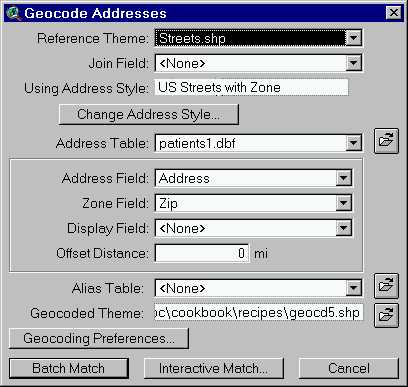
2. Notice that ArcView has automatically identified the appropriate fields in the street attribute table to use for address matching, as well as the appropriate method (U.S. Streets with Zone). It should have also selected "customrs.dbf" as the Address Table. Make sure this is the case. Also the Address Field should be Address, the Zone field should be Zip and the Display field should be Name. A new shapefile, geocd1.shp, will be created from this geocoding process. Notice that in the Geocoded theme field, the new shapefile, geocd1.shp, will be written to your working directory.
3. Click "Batch Match." ArcView will first build a geocoding index for the geocoding fields. The index will speed up the geocoding process. Next, it will do the address matching. When ArcView is finished it gives the percentage of matched customers (Unmatched customers are those for which it could not find addresses in the streets theme.) Note how many records from the customrs.dbf were matched with geographic locations in the geocoding process. You should be aware that in most cases the matching process is not as successful (as discussed in your textbook).
4. A resulting theme called "Geocd1.shp" will automatically be added to your view. Turn on the new theme to draw the customer locations on the map. This is the newly created point shapefile with each point representing the street address location of the customers in customrs.dbf.
5. Change the theme name to My New Customers.
6. Q: Compare the attributes of customrs.dbf with those of Geocd1.shp. How do they differ?
1. Choose the Select Feature tool. (Make sure the customer theme is
active).
(Make sure the customer theme is
active).
2. Using this tool, draw a box around the group of customer points in the census tracts with high average income by pressing the mouse at one corner of the box, dragging, then releasing the mouse button at the opposite corner of the box. All of the selected customers point locations will be highlighted in yellow in the View.
3. Display the attribute table for customers. The corresponding records for these selected customers are also highlighted in yellow in the attribute table.
4. Promote the selected records to the top of the table to more easily look at the information on the selected customers.
5. Now click on the "Sales" field name in the table to make it active.
6. Click the Sort Descending button to sort the customers with the
highest sales listed at the top, or select Sort Descending from the Field
menu.
to sort the customers with the
highest sales listed at the top, or select Sort Descending from the Field
menu.
7. Press the shift key while you click on the first five records in the table to select your top five customers. Notice your selected set has changed on the map as well.
8. Q: Where are your best customers located? Using the Identify tool (on the Tool bar), provide addresses AND latitude and longitude geographic coordinates for each customer. (hint: the coordinates are the pair of numbers found on the extreme right side of the tool bar).
9. Now make sure the Customer table is the active window so that you can ask a question for the table, or select Query from the Table menu.
10. Click the Query Builder button to display the Query Builder dialog
for the table, or select Query from the Table menu.
to display the Query Builder dialog
for the table, or select Query from the Table menu.
11. In the Field list double click on "Sales." It is added to the text window below, and will become part of the logical expression that defines your question.
12. Click once on the "greater than or equal to" operation button. The operator is added to the expression.
13. In the Values list double click on the nearest value to 55,000 (it is 55130.41) to add it to the question. You can also type the number 55000 (no comma) in the text window. Be sure to place the number between the operator and the closing bracket.
14. Click the New Set button to create a new selected set of customers. Notice how your selected set has once again changed on your map.
15. Close the Query Builder dialog.
16. Q: Within the selected set what is the address of the establishment with the lowest sales?
What is the address of the establishment with the highest sales?
How many establishments are movie theaters?
Note: You performed this query while the table was active, but you could also perform it using the same functions from the view window.
17. Clear the selected set of records by clicking the Select None button.![]()
You will now create a final map of your customers within the downtown Atlanta area.
2. From the Project window, select the Layout Document and open a New layout.
3. From the Layout menu, choose Page Setup. Change the Orientation to Landscape. The page size should be Same as Printer (11 X 8.5). Leave everything else the same.
4. From the Layout menu, select Add Neatline. Use the default values to add a border around the margin of the new layout. This cartographic element helps to define the area of focus and can also be used to group individual elements together within your map.
5. From the Tool bar, click on the View Frame button. Use the View Frame tool to create a frame in your layout for the map of Atlanta. In the View Frame Properties dialog, select the Atlanta View. Be sure that the Live Link box is checked and that the Scale is set to Automatic. Accept the rest of the default values
6. Again from the Tool bar, click on the View Frame button, hold and scroll down the icons until you find the Legend Frame button. Add a Legend Frame to your layout. In the Legend Frame Properties dialog, select the Viewframe1: Atlanta. Again, accept the rest of the default values.
7. From the Tool bar, use the Pointer Tool to select, move and resize the frames to fit on your layout page. With the Pointer tool, click on the cartographic element you want to select. Handles will appear around the graphic allowing you to move and resize it.
8. Continue to design your layout by adding a North Arrow (any style is fine) and a Scalebar using the appropriate frames for these cartographic elements. Remember to select the correct View Frame for the display of the Scalebar. You may change the style of the scalebar but remember that the distance units of our project are miles, so do not change this parameter.
9. Use the Text tool on the Tool bar to add a map title to the top of your map as well as your name to the bottom of the map. To change the text size, use the Pointer tool to select the title in your layout, if it is not already the selected graphic. Then from the Window pull down menu, select Show Symbol Window. The Font palette will open allowing you to change the font size. You can also change the style of the font if you wish.
10. Refine your layout until you are happy with the final results. Your final map should contain the following SIX (6) cartographic elements: Map, legend, title, north arrow, scalebar, and source statement including author and date and source of data.
11. An easy way to include your layout in Lab Report Word Document is to Export the layout to a standard graphic file format. To do this, with the Layout Document active, from the File menu, choose Export. In the Export dialog box, the default file type is a Placeable WMF (Placeable Windows Metafile), which works in Word. Specify a filename and check to make sure the file is being written to your working directory. Then click OK. In Word, from the Insert menu select Picture/From File and navigate to the saved file in your working directory to insert the graphic into your Word Document.
http://dusk.geo.orst.edu/arc/qstart2.html