LAB 1: Brushing up on ArcGIS 9
Instructions below updated for ArcGIS 9.3
Click here for ArcGIS 9.1/9.2 version
Suggested time for completion: One Week
Note: The assigned questions are in an MS-Word file from this link (Word document) or at the bottom of this document.
To re-acquaint with the following:
Computers
ArcGIS software is designed to run on
Windows XP. It can also run on Intel-based Macs using Boot Camp or Parallels.
About the software
In this course, we will be working with ESRI's ArcGIS
software. ArcGIS is considered to be the industry standard for
professional-grade
geographic information systems (GIS) users. In its current incarnation,
ArcGIS (version 9.x) is a Windows-based GIS program - a significant departure
from the structure of versions 7.x and below, which used command driven, DOS-
or Unix-based interfaces. While the latest versions of ArcGIS are Windows-based,
the software does include a copy of ArcInfo "Workstation," with essentially
the same structure as the previous command line versions of the software.
ArcGIS 9 is structured around three main modules: ArcCatalog, ArcMap, and ArcToolbox. These three modules perform the three basic functions of GIS - data manipulation, data analysis, and data output/mapping. In this lab we will cover these three modules in greater depth, as well as discover some of their key functionality.
Cartography
In this lab we will also discuss some basic principles
of cartography. For those familiar with cartography, or who have completed
prior GIS courses which involved creation of cartographic products, this will
likely be a review. This portion of the lab will provide you with the
basic guidelines and requirements for all maps and cartographic products handed
in with lab assignments.
Additional information
Additional information on the ArcGIS software can
be found through
ESRI's ArcGIS 9 web site, and through the ESRI
Virtual Campus web site, which offers several modules on ArcGIS, ArcGIS
extensions, and other ESRI products. Oregon State University has
the good fortune to have an ESRI site license that gives access to a number
of ESRI virtual campus courses. Complete information on the about our site license can be found at geo.oregonstate.edu/esri.
The data that we will be using in this lab are:
Geodatabases:
Download the data here (3.7 Mb) into your local work folder.
1.4.1 The Basics
1.4.2 ArcCatalog
ArcCatalog is the ArcInfo module used for organizing,
browsing, and managing your data and map files, as well as for viewing and editing
metadata. In many ways, ArcCatalog is similar toWindows Explorer. For
instance, when you modify a file's location, or create or delete a file, you
do not need to save the changes -- it is done automatically. Since it is easy
to delete files this way, you should be careful to delete only when you are
sure that you will not need the file any longer.
| Answer question 1: What is the function of each of the following buttons? You will run into these icons as you go through the lab: |
| Connecting to your data
To access your data in ArcCatalog you have several choices -- first, if there is already a connection to the drive with your data, you can navigate down the catalog tree until you find your data folder. This, however, has the potential for causing quite a bit of clutter and confusion if your data are more than one or two folders down from the drive connection. A second option is to create a direct connection to your data. A direct connection will help avoid clutter; you can make a connection straight to the folder holding your data, rather than having to navigate through other folders -- it is also a necessary step if the drive with your data are not shown in the Catalog tree (i.e.,if you are using data saved on your network drive). An example of a direct connection can be seen in the graphic in section1.4.2. -- G:\nicktemp and G:\sarah are both direct connections to local data folders.
Try this out and connect to your network drive, or to the local folder that you will be using for your work.
|
| What can I do in ArcCatalog?
Earlier in the lab, it was mentioned that
ArcCatalog is used for "organizing, browsing, and managing your data
and map files, as well as for viewing and editing metadata." Let's
explore that a bit more: For organizing data, ArcCatalog is quite easy to use. However, if you delete, move, or otherwise alter the data using ArcCatalog, it is permanent (i.e., if you delete a coverage, it is GONE - you can not retrieve it). Data organizing in ArcCatalog is very similar to that in Windows Explorer - you can drag and drop coverages, shapefiles, or geodatabases into new workspaces, or you can use the Windows shortcut keys (CTRL-C and CTRL-V). Try this out by copying and pasting your lab
data into a new folder. Browsing through your data are simple using ArcCatalog - the Catalog tree displays in a hierarchical fashion all of the items in the Catalog - much like data browsing in programs such as "Windows Explorer." A folder that contains files will have a box with a plus or minus sign to the left of the file name. This indicates whether or not the folder has been expanded. Take a moment or two to explore the data in the Catalog tree - you can use the arrow buttons on your keyboard, or your mouse to navigate. While navigating, pay attention to the changes that take place on the right hand side of the ArcCatalog window.
The right hand side of the Catalog allows you to examine the data further. For instance, select the lower48 coverage and click on the "Contents" tab on the right hand side of the window. You will see a list of the files that comprise the coverage. You can also see these files if you click on the plus sign to the left of the lower48 icon. If you click on the "Preview" tab, you will see a preview of the data geography or the data attribute table. To change from geography view to table view (or vice versa), change the value listed in the preview pulldown menu at the bottom of the Window. |
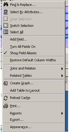
| Answer question 2: When previewing data, a new set of icons become
active in the menu bar. Why? What do they do? Are they
always active when previewing data?
Answer question 3: Do you find the preview tab helpful? Why or why not? |
Finding data in ArcCatalog
As well as finding data, you can also add
fields to the table, re-load the table to view recent changes, or export
the table as a .dbf file (dBase IV format, a format readable/importable
by most spreadsheet and database programs, including Microsoft Excel),
and the native format for Shapefiles. The coverage's native format is the
INFO table. |
| Answer question 4: Using the uscnty shapefile, find the state or states to which the following counties belong. Note that there may be more than one state with a county of that name.
|
| What can I do in ArcCatalog? (cont.)
Using the lower48 coverage, if you select the "Metadata" tab you will see any metadata (or data about the data) that is associated with the coverage. No metadata has been created for any of the data that we are using in this lab, so most of the metadata file is not filled in. ArcInfo automatically fills in a few fields in the metadata -- under the Spatial and Attribute headings. In a later lab we will be creating our own metadata. |
| Answer question 5: Why do you think that these fields are automatically filled in, and the fields under the description are not? |
| Managing your data Managing your data is also done in ArcCatalog. You can examine and/or modify the properties of your data simply by right-clicking on the coverage, shapefile, or geodatabase and selecting Properties. Try this with the lower48 coverage file.
On your own, explore the property sheets for
each of the feature classes for lower48. To do this, expand
the lower48 coverage by clicking on the plus sign
next to the coverage icon, right-click on the one of the feature
classes (arc, polygon, tic, label), and select Properties. |
| Answer question 6: What spheroid is the lower48 shapefile using? |
Introduction to ArcToolbox
ArcToolbox is the ArcInfo module used for data processing,
analysis, and conversion. ArcToolbox also provides an option for the user
to write scripts and create customized data processing/analysis/conversion tools.
| Starting ArcToolbox To start ArcToolbox, you can either open it through the ArcCatalog or ArcMap interface. On the ArcCatalog main toolbar, click on the |
| The lay of the land, or, What is in ArcToolbox?
As you can see when looking at ArcToolbox, it provides tools for geoprocessing - data management, analysis, and conversion. There is also an option called "My Tools" which allows the user to create new, custom tools or run scripts. Let's explore the organization of ArcToolbox a bit more:
|
| Answer question 7: Use the toolbox "Search" tab (located at the bottom of the ArcToolbox dockable window) to find all tools related to "overlay" operations regarding coverage tools. List these tools along with a brief description of their function. |
| Introduction to ArcMap
ArcMap is the ArcInfo module used for creating,
viewing, querying, editing, composing, and publishing maps. You will
be spending a lot of time using ArcMap. Starting ArcMap Similar to ArcToolbox, ArcMap can be opened
via the Start menu (Start -> Programs -> ArcInfo -> ArcMap) or from
ArcCatalog(click on the When you first start ArcMap, you may see the"Welcome to ArcMap" window - this window provides the options to 1.) Create a new map, 2) Open the last map you were using, 3) Open an existing map,or 4) Create a new map using a map template. This quarter we will most often use options 1 and 3 (creating a new map, and opening existing maps). If you do not see the Welcome window, someone
has probably turned this option off - don't worry, you can still access
all of the options through the main menu. For the sake of
description, open the prepared map file provided with the lab data (BentonCoMap.mxd
)- you can open this from the Welcome window, or when ArcMap is open,
click on File -> Open File, and navigate to the location of the map
file. You will notice that the BentonCoMap file is not particularly
stunning from a cartographic standpoint. Later in the lab, you
will fix up the map to make it a bit more cartographically pleasing.
The lay of the land, or, What is in ArcMap?
The left portion of ArcMap shows a tree displayof
the layers (the "layer tree") added to the map (and whether or not they
are currently displayed). There are two ways which the included
data can be explored - by "Display" or "Source." You can toggle
between the two by selecting the appropriate tab on the bottom of the
layer tree: The right portion of ArcMap provides a view
of the data (similar to ArcView). You can select to view the data
in "data view" or in "layout view". At the bottom of the view window
three very useful icons appear. In the data view, you can zoom in and out,
pan, identify, select, etc. the data in this portion by using the available
tools: |
| The lay of the land, or, What is in ArcMap? (Cont.)
After exploring the data view, go to the layout view - you can do this by either clicking on the sheet of paper icon at the bottom of the view window, or by selecting View->Layout View. The layout view is similar to the layout in ArcView. A new set of tools are provided for exploration of the layout: 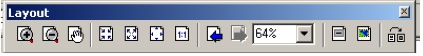
To insert a title, legend, neatline, etc. on your map, click on Insert and select the object that you would like to add. Experiment with adding information to your map - try adding a title, legend, scalebar, north arrow, and your name. You will use this map file later in the lab, so you will want to save your changes either in a new Map file, or overwriting the one in your directory Note- The Map file does not contain
data. It contains information about how your map is layed out, and what
data is in your map - You could think of your hard drive as a kitchen,
map files as your recipes, the data as your ingredients, and the software
as a cook. You write the recipe, or even change it, but the dirty work
of baking and cleaning is the responsibility of the cook. (And that
makes you the Master Chef....) Adding data / creating your own map Now that we have spent some time with an already created map file, let's make our own. In ArcMap, you can not have two map files open at the same time, so to open a new map file we either need to open a new ArcMap window or close the existing map file. In this instance, since we will not need to use the BentonCoMap for this portion of the lab, click on File --> New (or you can use the shortcut key "CTRL-N" or click on the new file button on the menu bar), and select "Blank document." To add data to a map file, there are several options: 1. Use the "Add data" button on the ArcMap toolbar Try each of these methods, and add the lower48 coverage, and the uscnty,usroad,and usriv shapefiles to your new map file. Since it is likely that you will open data from both your network drive or from copies on a local drive (zip or cd), it is helpful to use a "relative path" to your data rather than an 'absolute path'. This will be handy if you copy your lab data folder to a local drive to work, or if you move it from one drive to another - if you do not store your data sources with relative path names, you will run into the problem of ArcMap looking for the data on the last drive that you used with that particular map - one that might not exist on the computer you are working on. For example, a map created with data located in D:\lab1 will be searched for in D:/lab1 regardless of where the data actually is if an absolute path is used. To continue the cook analogy above, the software(cook) looks for the ingredients (data) at the location specified in the recipe(map file). The absolute location might be "on the third shelf of the refrigerator". If the ingredients are moved, the directions are no good, but the recipe can move around anywhere. The relative path name tells the software to look for the data in the same relative location to the map file- e.g., in the same location relative to the recipe. So if you keep your recipe with your ingredients, you can move them both to any location you like, and the recipe is still valid.) To set your map file to use relative path names, click on File --> Document Properties, select Data Source Options,and "Store relative path names." Click OK. Note: You will probably want to do this with ALL map files that you create in this course. Because you may shift computers or even computer labs, you will be able to transfer the folder, with its files to any location you want. Occasionally, even if you set the map file
to use relative path names you will still have problems with "broken
sources." These will be indicated by a red
! next tothe layer's name: To fix this problem, go to Properties-->Source
,and re-set the appropriate data source by clicking on the "Set Data
Source" button. Symbology and data appearance
Data properties: In ArcMap, to view the properties of a data
layer, double click on the data layer's name. This
will take you to the properties window. Note: The ArcMap properties
window will provide different information than was found in the
ArcCatalog Properties window. You can also do this by right
clicking on the data layer and selecting the properties option.
From the properties window you can view and modify the display properties
of a dataset - including the layer's transparency, labeling options,
symbology, and source. This lab will only cover a few of the options
(display, symbology, and labels), but you will want to take a few moments
to familiarize yourself with the other functions in the properties window.
Symbology: Under the symbology tab are the options for changing the display of data. From here you can decide to display the data as Features (single symbol), Categories (unique values, unique values many fields,or match to symbols in a field), Quantities (graduated colors, graduatedsymbols, proportional symbols), or Multiple attributes (quantity by category). You can also decide what color(s) and symbol(s) to use to represent thedata. For example, if you want to use usroad
to display type of road rather than simply a location - double click
on usroad to open the Properties window, and click on
the Symbology tab. As the default, usroad is drawn
as a single symbol -since we want to show all of the different road
values, we will use Categories-->Unique values. Let's divide
|
||
| Answer question 8: What information is provided in the symbology tab when we select the ADMIN_CLASS field? From this window, in what ways can we change data representation? |
| Symbology and data visualization (Cont.)
To change the representation of Interstate,
State Highway, and US Highway, double click on the line next to the
name and select an appropriate line symbol from the Symbol Selector.
Change to appropriate symbols. Since there are no "other values,"
you can deselect the 'all other values' symbol. When the display
is to your liking, click OK. Display An important feature on the display tab is the option to set transparency. This allows for a layer to be seen through another layer - for instance, with the uscnty layer displayed, the lower48 layer can not be seen. By setting the top layer to some level of transparency, both layers can be seen. With the transparency function, you can even display a raster layer transparently to give a 3-D effect! To explore this, we'll make the uscnty layer partly transparent. Open the properties window for uscntyand select the Display tab. Under "% Transparent" enter 75 and click on OK. Now the state boundaries are shown clearly, and the county boundaries are less pronounced in the display. |
| Answer question 9: Where else do you think the transparency function might be (more) useful? |
| Labels
Using the labels tab under properties is an easy way of inserting the names of features on a map. We will try this out with the usriv layer and add labels for river names. Go to the labels tab in the usriv property window. To insert labels, check the "Label Features" box and select which field to use for labeling (we will use "Name"). From here you can change the style, symbol, font, font size, and location of the labels by selecting from the button options under "Label" in the window. Take a few minutes to explore these options. |
|
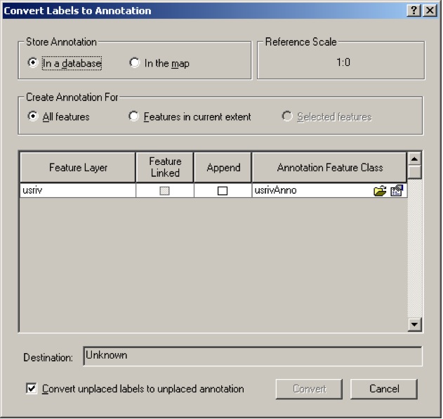
Now try to move or delete only ONE of the labels... Can you? The problem is that the labels are based on a specific feature value, and a point defined by the feature. To change individual labels, they must become a special kind of graphic, ones attached to points in a seperate layer within your rivers shapefile called an annotation layer. This way the points can be changed individually, but still follow around the rivers layer. Right click on the rivers layer in the table of contents, and Convert Labels To Annotation. Use the Default settings, but select In the map for Store Annotation.. Hit Convert, and using the arrow tool, try to select and move one of the new annotations. This is far easier than maintaining them as automated labels. What happens to the labels when you change the scale of the map by zooming in or out??? What if you want labels that are not attached to your rivers layer??? Or if you want to change the thickness of a single segment of your rivers??? Once again, right click on the rivers layer and look at the option to convert Features to Graphics and think about what it might be good for.. DONT USE IT AT THIS TIME. |
| Answer question 10: Describe the differences between automated labels, the annotation layer and graphics. (briefly) |
Querying data in ArcMap
Choose the Select By Attributes option, and then write a query to select the counties that meet the following criteria:
When doing searches of this type, it can be
handy to display only those records selected. To do this, change
the option to show selected: Notice that the selected counties are highlighted not only in the attribute table, but on the display map. |
| Answer question 11: In which state is the selected county? Write out (as you typed it) the formula that you used to find the answer. |
| The (VERY) Basic principles of cartography
ELEMENTS: 1. Data in maps: 2. Titles: 3. Scalebars: 4. Borders: 5. North Arrows: 6. Legends: 7. Text on Map: 8. Source 8. Name on Map: 9. White Space: PRINTING: 2. Don't wait until the last minute to print!
|
| Your maps for Lab 1: Map 1- Using the lower48, uscnty, usriv, and usroad data, zoom to your favourite state and make a map of it. Follow the above listed principles of cartography. Include whatever features (rivers, roads, counties) you feel are necessary (at least one must be included). Turn in this map with your lab answer sheet. Map 2- |
As with any new software, these basics do not come close to being comprehensive, however - to really grasp the software, you will need to spend quite a bit of time just exploring, trying out different functions, seeing what works (and what doesn't), and just clicking on buttons, menus, bits of data, and especially the help files.
In the remaining labs this quarter, we will spend time examining more specific GIS functions with ArcGIS Desktop 9.x
Consider turning in one MS-Word document with screen shots of the maps inserted directly into the document.


 the
road by administrative class (Value Field = ADMN_CLASS). To add
these values to the display, select "Add all values." If you do
not want all of the values to be displayed, you can add values individually
using the "Add values" button. To change the symbology of other
data layers (even of other types of data -- shapefile, coverage, or
geodatabase) the process is the same. Note that you can also alter all
the values at once, by clicking on the symbols column heading.
the
road by administrative class (Value Field = ADMN_CLASS). To add
these values to the display, select "Add all values." If you do
not want all of the values to be displayed, you can add values individually
using the "Add values" button. To change the symbology of other
data layers (even of other types of data -- shapefile, coverage, or
geodatabase) the process is the same. Note that you can also alter all
the values at once, by clicking on the symbols column heading.