Increasingly, anthropogenic pressures such as over-fishing, coastal development and aquaculture have degraded habitat and put marine resources at risk (Leslie et al., 2003; Mumby et al., 2001; Puniwai et al., 2003). In response, there has been a growing interest by resource managers, policy makers and academics in the use of marine protected areas (MPAs) as a management tool to help slow, prevent or reverse negative anthropogenic changes. Currently, more than 100 MPAs have been established worldwide; however, these protected areas encompass less than 1% of the world's oceans, less than 1% of U.S. waters (PISCO, 2002) and less than 1% of the main Hawaiian Islands (Tissot et al., 2004). Yet, despite the small amount of area protected, the most recent scientific research suggests that MPAs considerably enhance the conservation of marine biodiversity and contribute to the management of marine fisheries (e.g., Carr et al., 2003). These studies show that MPAs meet the economic and social needs of fisheries and communities dependent on ocean resources by protecting spawning grounds and increasing the abundance of fish stock in adjacent areas due to spill-over effects (e.g., Christensen, 2003). MPAs also preserve ecosystem components, such as habitat, food and shelter, which are critical to fish growth and survival. Furthermore, MPAs in Hawaii have been demonstrated to effectively promote the recovery of fish stocks depleted by fishing pressures, without significant declines outside of reserves (Tissot et al., 2004). Thus, MPAs offer potential management solutions for resource protection and the prevention of over-exploitation. But can the effectiveness of the MPAs be increased by examining spatial near-shore reef fish and habitat information?
This study begins to address this question by using the Marine Data Model (MDM) (Wright et al., 2001) to integrate available near-shore fish species information from private and public sources around the main eight Hawaiian Islands. By integrating spatial information on near-shore fish species into the MDM, patterns of spatial habitat utilization and gaps in conservation were identified. The study of habitat utilization patterns is important because of the relationship that exists between fishes and their habitats (Christensen, 2003). By determining which combinations of habitat types are necessary for survival, the efficacy of the network of MPAs in West Hawaii can be evaluated. Additionally, this study used the querying ability of the MDM to evaluate the habitat utilization patterns of specific near-shore marine fish along the west coast of the island of Hawaii (hereafter, West Hawaii) by identifying correlations between regional scale (large-scale) spatial information and fine (small-scale) spatial information. This is important because available scientific research has not evaluated the current status of near-shore marine habitat utilization in West Hawaii at the large scales utilized by resource managers. Typically, most marine studies have been conducted at very small-scales; however, management units are usually on the scale of an island or an entire state and resource evaluation should reflect this scale (Friedlander and Brown, 2003).
The MDM is a data model tailored specifically for the marine community. Created by researchers from Oregon State University, Duke University, NOAA, the Danish Hydrologic Institute and ESRI, work on the data model began in 2001 and resulted in the first major draft of the MDM. This model was created in response to three major needs by the marine GIS community: (1) provide an application-specific geodatabase structure for assembling, managing, storing and querying marine data in ArcGIS, (2) provide a geodatabase template to meet the needs of a specific community of users, and (3) provide a better understanding of ESRI's new geodatabase data structure. By using the MDM in this case study the model was tested to determine its adaptability in working with real-world data and performing real-world analyses, as well as identify its strengths and weaknesses in meeting three major needs of the marine GIS community:
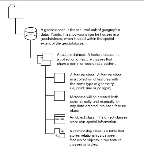
The ArcGIS MDM was designed to be used as a geodatabase template for marine GIS users. The geodatabase template, like all geodatabases, is an organized hierarchy of data objects. These data objects are a collection of feature data sets, feature classes, object classes and relationship classes (Figure 1).
Specifically, a feature data set is a collection of feature classes that share a common spatial reference. The spatial reference is part of the definition of the geometry field in the database. Accordingly, a set of transect survey points stored in the coordinate system NAD84 UTM Zone 4 could not be in the same feature data set as geographic latitude/longitude coordinates. In the geodatabase, all objects represent a real world object such as a marker buoy or lighthouse, and are stored in a row in a relational database table. Object classes are not represented geographically; however, they can be related to spatial information through a relationship class. Conversely, all of the features in a geodatabase are geographic objects that have a defined spatial location. Basically, a feature is just like an object but it also has a geometry or shape column in its relational database table. The hierarchical data structure of the geodatabase allows the feature classes to inherit all of the attributes and behaviors of the object, but retain the spatial capabilities (Zeiler, 1999). The MDM geodatabase can store a range of data sets, from the small to medium data sets of personal geodatabases, to the very large geodatabases managed with the help of ArcSDE (Arc Spatial Database Engine).
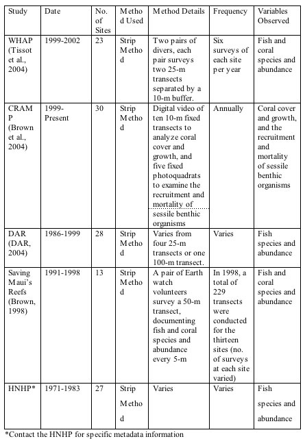
Fish transect survey data from Hawaii were obtained from various federal, local and academic institutions through the Hawaii Natural Heritage Program (HNHP). The data were gathered and organized in a Microsoft Access relational database which was used primarily for its querying abilities and large data storage capacity. The data gathered were from: the West Hawaii Aquarium Project, the Coral Reef Assessment and Monitoring Program (CRAMP), the state of Hawaii's Division of Aquatic Resources (DAR), the Saving Maui's Reefs project and individual peer-reviewed journal articles input into a database for the HNHP (Table 1).
Table 1.
The dates, sites and survey methodologies of fish survey data used in each study. Note: WHAP and Saving Maui's Reef projects also focus on obtaining coral information; however, this study excluded that information from the database. Also, information on sessile organisms from the CRAMP data set was included in this database because this information will be later used by the HNHP in their larger MGAP project.
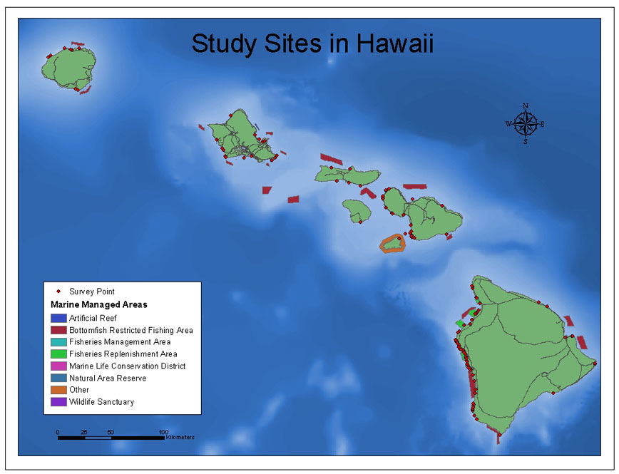
The data sets obtained through the HNHP contains information on 121 sites located throughout the main Hawaiian Islands (Figure 2). These sites are located in 15 different habitat types and 5 zones, and are located in areas with different levels of protected status (NOAA, 1999a).
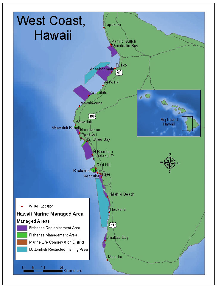
The area examined in the habitat utilization analysis is the West Coast of Hawaii Island (see Figure 3). From Lapakahi to Manuka this study represents approximately 212 sq km of shoreline, fifteen different habitat types and five reef zones. This area was chosen due to the availability of fish transect survey data and habitat information.
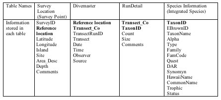
ll data sets were combined into a single MS Access database created to store these data. This database consisted of four primary tables: (1) survey location information, (2) Divemaster (3) RunDetail and (4) species information (Table 6 for specific information). All tables had a key field that was used to relate one table to another, allowing the user to query related information throughout the tables. This database design allows for queries involving variables of space, time, and fish species.
Table 2. The database structure of the combined Hawaii reef fish database.
Testing the well the MDM met the three needs:
1 and 2: Provide an application-specific geodatabase structure for assembling, managing, storing and querying marine data in ArcGIS, and provide a geodatabase template to meet the needs of a specific community of users.
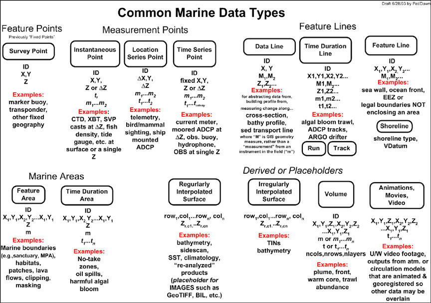
In the MDM, the feature data sets and classes cover a very broad range of marine applications (Blongewicz and Wright, 2003) (Figure 4). For example, the marine feature data set contains seven feature classes used to store information representing physical maritime features such as natural or manmade objects in the water. One of these feature classes is the SurveyPoint. The SurveyPoint feature class in the MDM was used in this case study to store the x, y, and z locations of survey points. This feature class was used because it was set up to store information on features that have fixed x, y and z coordinates. Accordingly, each point in the SurveyPoint feature class represents a 3D location where a transect survey was conducted. It should also be noted that many survey point locations in this case study represent only an approximation of the location where the fish transect survey was conducted, as the exact latitude and longitude coordinates are unknown. However, the information recorded in the geodatabase reflects the best possible estimate.
Before any data were added to the geodatabase, the spatial extent and the projection of the feature classes were established. This was done by importing the NAD83 UTM Zone 4 projection information and spatial extent from a polygon shapefile of the main Hawaii islands (DBEDT, 2004) into the MDM. Accordingly, all subsequent shapefiles imported into the geodatabase would need to be in the same projection (ie, NAD83 UTM Zone 4), and fall within maximum x, y spatial extent.
The Access table containing the transect survey latitude and longitude coordinates was then imported into ArcGIS 8.3. Using the create x, y function, a point shapefile was generated. This 2D shapefile was converted into a 3D shapefile using the z values (depth) in the attribute table. This was necessary because all shapefiles imported into the SurveyPoint feature class must be 3D in accordance with the established model parameters, even if the 3D values do not exist.
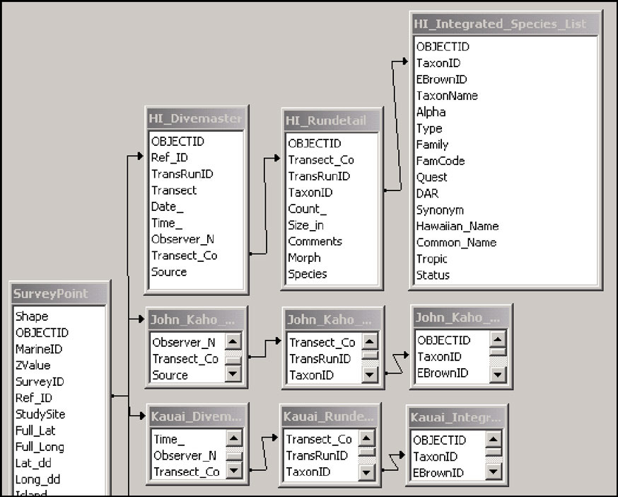
It was initially thought that the SurveyPoint feature class could be further defined with information stored in the SurveyInfo object class. However, due to the large amount of data, this did not prove to be possible. With over 250,000 entries, if all of the data were combined into one table representing the main Hawaiian islands, it would take the MDM over 2 hours to perform one query. Thus, by separating data by island, queries could be conducted in less than one minute, and multiple queries could be conducted if information on more than one island was needed. As a result, the MDM was personalized to fit the data in this analysis. To personalize the MDM numerous field names and tables were added to the geodatabase. The added tables were: Divemaster, RunDetail and Integrated Species, which were specific to each island (i.e., Oahu Divemaster, Hawaii Rundetail, ect). These tables further describe the SurveyPoint feature class by providing information like survey dates, who conducted the survey, and which species were observed along transects.
When all the data were entered into the geodatabase, relationships were established between the feature classes, or spatial information, and the tables, or non-spatial information (Figure 5). These relationships consisted of one-to-one and one-to-many relationships. A one-to-one relationship matches one entry to an identical entry in a separate column/table. A one-to-many relationship matches one entry to multiple identical entries in a separate column/table. Additionally, due to the nature of the geodatabase, these relationships are permanent and unlike joins, will not have to be reestablished in each new project.
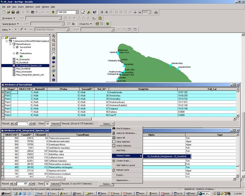
One of the main reasons the MDM was used in the habitat utilization analysis was due to the ability of the model to easily and efficiently query for spatial information. Accordingly, the established database design allows for queries involving variables of space, time, and fish species. Thus, by querying the MDM, the site locations where a specific fish species has been observed (Figure 6) can be determined. These sites are then overlaid on large-scale habitat types to determine what species were found in what habitat types.
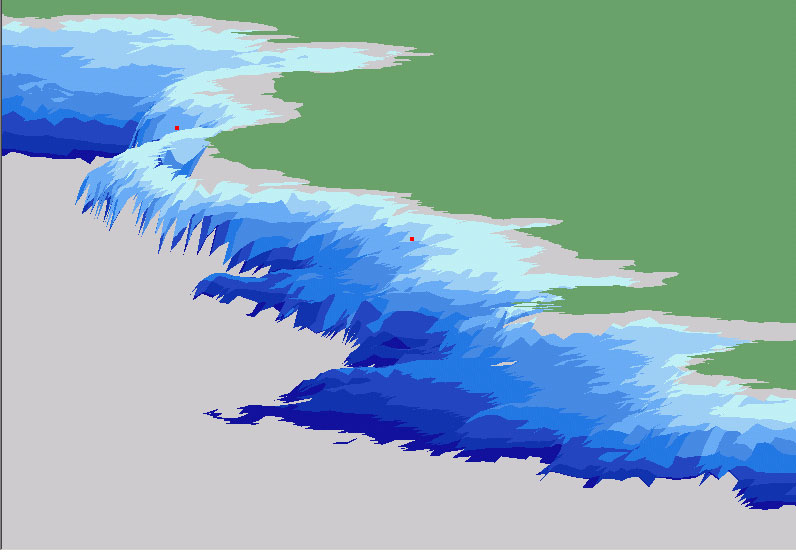
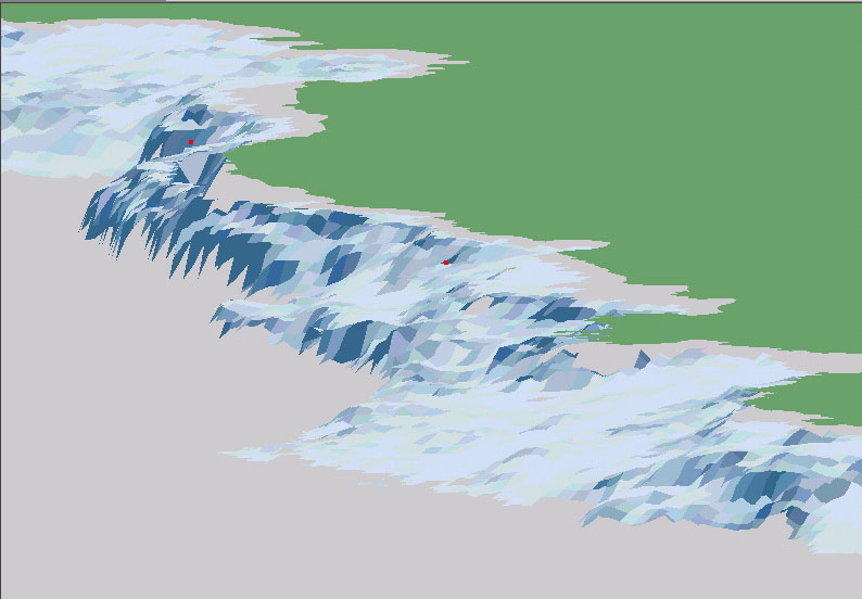
The data were also mapped in ArcScene to better observe the data in 2.5D. Viewing the data in 2.5D is particularly helpful when examining the location of the survey points in relation to the bathymetry and rugosity layers (Figures 7 and 8). In a 2D view, the location of the Puako survey site on the edge of a drop-off is not as apparent as it is in the 2.5D view. This visualization can aid greatly in understanding the ecological differences in flora and fauna found at Puako vs. a site like Anaehoomalu which is located on a gentler slope.
3: Provide a better understanding of ESRI's new geodatabase data structure.
Due to the rapid development of GIS software, many users are still working in ArcView. To help users become more familiar with GIS in general, and more specifically with the geodatabase model, a tutorial describing how to use the MDM was created as a part of this research. Graduate students in the Davey Jones Locker Seafloor Mapping & GIS Laboratory at Oregon State University who have used the MDM tutorial describe it as easy to use and understand, particularly with regard to the diagrams and the formatting.
The WHAP data set was used because it is one of the most comprehensive and statistically robust Hawaiian reef fish data sets. Additionally, it covers twenty-three sites along the West Coast and it spans a multi-year time period. The detailed steps taken to answer each of the three sub-questions are outlined below (Figure 9).
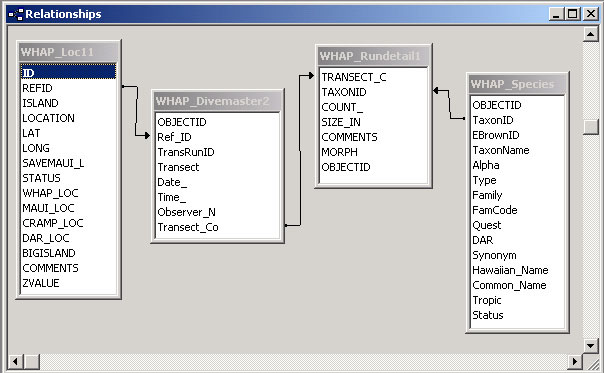
In order to analyze the WHAP data set in this analysis, the MDM was used to query and separate the WHAP data from the other data in the geodatabase. It was necessary to isolate data specific to WHAP, so as not to confuse a fish species observed on a DAR survey at the same site as fish species observed on a WHAP survey. Moreover, it was important to separate the WHAP data because survey methodologies differed between data sets, because an analysis of a compilation of data sets would not be statistically valid. When the data were separated, a new feature class called Whap Location was created, along with 3 tables: Whap Divemaster, Whap Rundetail and Whap Species. All of these data remained in the MDM, and new relationships between the tables and feature class were formed following the initial MDM database design (Figure 10).
To determine the habitat type and zone for each of the WHAP sites, the WHAP Location feature class was overlain on a NOAA's large-scale benthic habitat layer (Figure 14). Using the select-by-location function in ArcGIS, the habitat types and benthic habitat zones for each of the WHAP sites were determined.
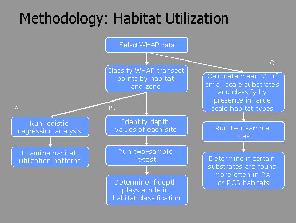
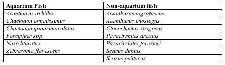
Once each WHAP site was classified according to habitat type and zone, a logistic regression analysis was used to determine the pattern of habitat utilization of six aquarium and seven non-aquarium fish species (Table 3) between the different habitat types. These fish species were selected because they represent commonly collected aquarium and reef fish observed during WHAP surveys.
Table 3. Aquarium and non-aquarium fishes examined.
Following the methodology outlined by Christensen (2003), a logistic regression was used to fit a model to a binary response (Y=1 if present or 0 if not present) to the independent variable (X=habitat type), such that for each column, there was a probably p of being present or p-1 if not being present. The MDM model was used to query the location of each specific fish to determine its presence or absence at each WHAP site.
Further analysis into the habitat utilization of specific fish species was conducted to determine if there were correlations between the small-scale substrate information gathered in 1999 by the WHAP researchers (Tissot et al., 2004) and the large-scale habitat information delineated by NOAA in 2000 (NOAA, 1999a). To do this, the mean percentages of each small-scale substrate type found at each WHAP site were calculated. The WHAP sites were then categorized according to habitat type, and the information was compared using a two-sample t-test.
To determine if depth values played a role in the classification of NOAA's large scale habitat types, the depth values of each of the WHAP sites were determined. The WHAP sites were then categorized by habitat type and the information was compared using a two-sample t-test.
Rugosity Layer. The rugosity layer was mapped using the Scanning Hydrographic Operational Airborne Lidar Survey (SHOALS) data from the US Army Engineer District (SHOALS, 2000). The SHOALS data were collected in 2000. The LIDAR data were used to derive both the bathymetry, as well as the rugosity grid. Both of these grids were clipped to exclude areas that overlaid land or were located in the intertidal zone. Rugosity was determined by using the ESRI script, "Surface Areas and Rations from Elevation Grids." This extension calculates the rugosity by dividing the seafloor area by the surface area (ie, a value of 1 equals a completely smooth sea floor). This calculation is much like the chain link method, where the transect chain length at the bottom is divided by the chain length from the surface; however, this method calculates the value for an area as opposed to a single transect line (Jenness and Engelman, 2004).
Another goal the working group sought to address was to provide, for the marine GIS user community, a better understanding of ESRI's new geodatabase data structure. The results of this analysis have shown that in conjunction with the tutorial, this goal has been met. Colleagues at Oregon State University who have used the tutorial to become more familiar with the MDM state that it is easy to use and understand. Also, they state that they have become more familiar with tool placement and analytical capabilities in ArcGIS. In addition, for those users with very little geodatabase experience, working through the tutorial will familiarize them with terms and concepts associated with geodatabases, as well as show them how to work with geodatabases. We look forward to more feedback from the user community as the tutorial is used more widely.
Table 4. WHAP study sites categorized by habitat type.
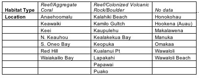
From this table, it can be seen that seven sites are located in the RA habitat type, nine sites are located in the RCB habitat type, and seven 'no data' sites which do not have a habitat classification because NOAA's benthic habitat layer does not cover all areas along the West Hawaii Coast. The RA habitat type is defined as, "coral dominated formations with high relief and structural complexity. [They] often serve the same role as linear reef in fringing reef systems where the reef crest is relatively unorganized" (Battista, 2003). The RCB habitat type is defined by NOAA as "solid volcanic rock that has coverage of macroalgae, hard coral, zoanthids, and other sessile invertebrates that begins to obscure the underlying surface" (Battista, 2003).
Once the WHAP sites were categorized by habitat type, a logistic regression was used to determine the habitat utilization patterns of the selected reef fishes (Table 5).
Table 5. Results of logistic regression for individual aquarium fish species.
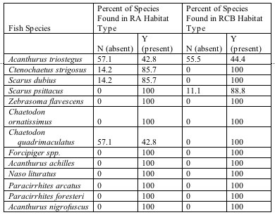
These results show that there is little habitat utilization preference between the RA and RCB habitat types for these selected species. A slight preference for the RCB habitat type is observed, but further studies are needed to verify these results.
To determine if certain substrate types were significantly more abundant in the RA verses the RCB habitat types, the mean percentages of each small-scale substrate type were compared using a two-sample t-test (Table 6).
Table 6. Mean percent cover for the WHAP substrate categorized by RA and RCB habitat types. * Indicates significance (p<.05).
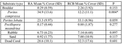
These results show that Porites compressa (finger coral) was significantly more abundant (p<0.05) in the RA relative to the RCB habitat types. In addition, the Porites lobata (lobe coral), while not significant (p>0.05), shows a strong trend toward being found more often in the RCB habitat type.
An additional analysis was conducted to determine if depth played a role in the large-scale habitat classification. The depth values of each site were compared to the classification of the site habitat as either RA or RBC using a two-sample t-test. The mean depth value of the RA habitat type is 41.71 '/- 5.77m, and the mean depth value of the RCB habitat type is 37 '/- 3.65m. The result from two-sample t-test shows that while depth values are not significantly different (p=0.088) between RA or RCB habitat types, the trend indicated that RA habitats occurs deeper than RCB habitat types.
This analysis has shown that the MDM has been used successfully for the analysis of habitat utilization patterns of reef-fish, with some insight gained as to how the model could be modified to better meet the needs of the marine community. In addition, the MDM is a versatile tool that can be used to perform a variety of functions for marine users. Not only can it store, assemble and query data, but it serves as a tool for examining spatial patterns of marine data at both a large and small-scale. However, this analysis has also shown that the MDM is best suited for two types of users. The first user is one who has never used a geodatabase before. For these users, the model provides a template with complete instructions in the form of a tutorial, on how to propagate the MDM with data. This saves the time it would take to learn how to design a geodatabase from scratch. And the second type of user has prior experience with GIS and can take advantage of object-orientation. This is because much of the analytical power behind the MDM is a result of the object-orientation functionality, which takes prior programming knowledge to fully utilize.
Ideally, the users would have a variety of marine data types to store in the geodatabase, which means that more than one feature class would be utilized. This ensures that it will be worth their time to use and personalize the model to suit their needs. On the other hand, the user would not have a great quantity of data, as the speed of queries depends on the amount of data stored in the geodatabase tables. For example, one of the tables in this study contained over 250,000 data entries. To query through the table it took the MDM over two hours.
To allow users to take advantage of the object orientation capabilities of a MDM geodatabase, it is suggested that a template for some behavioral and validation rules be included with the model. This will make the use of object-orientation in the MDM easier and more assessable to the average marine GIS user. This in turn will allow the marine community to better take advantage of the object orientation capabilities, which would greatly increase the analysis and modeling capabilities.
When studying the regional habitat patterns for selected reef fish, the logistic regression showed a slight habitat preference between the RA and RCB habitat types. This is likely due to the fact that NOAA's habitat layer is very generalized, as the habitat classification shows only continuous habitats greater than 1 acre in size (Battista, 2003). The lack of finer habitat information points to a need for further research into providing more detailed habitat information at a scale between NOAA's benthic habitat delineation and WHAP's detailed substrate information. If this was available at the time of this study, it is speculated that the results for the habitat utilization pattern might have been different.
This study also found that RA habitat is highly likely to be found at deeper depths, while RCB tends to be found at more shallow depths. Additionally, the coral Porites compressa was found significantly more often in RA, while Porites lobata was found more often in RCB. This means that Porites compressa will more likely be found at deeper depths than Porites lobata. This result is consistent with other data analyzes that have found finger coral to dominate most areas of the West Hawaii coast at 10-18m depths except along exposed headlands and recent lava flows (Dollar, 1982 and Tissot et al., 2004). This is important as finger coral provides an important habitat for juvenile aquarium fish, especially the Yellow Tang (Zebrasoma flavescens) (Tissot et al., 2004).
Results of the habitat analysis also showed that correlations existed between habitat information at two different scales. This result has important management implications as most marine management units are on the scale of an island or an entire state, whereas most ecological studies are typically conducted at a small-scale. Currently, the lack of detailed habitat information is a result of the high cost and time it takes to conduct a detailed survey. Thus, this study is important not only because it bridges the scale gap but it provides a new level of information to the large-scale habitat layer without high cost or time consuming surveys.
This study has also shown that depth is an important factor in habitat location. From a management prospective, this is important when looking at the boundaries of the protected areas and examining how far they extend into deeper waters, as previous studies have found that the more effective protected areas for specific species have boundaries that extend into deeper water (Tissot et al., 2004). For example, as Porites compressa was found more often in the RA habitat, and this coral is known to be a critical habitat for the Yellow Tang, it is important for managers to evaluate the protected area boundaries to ensure that RA habitat is also included in the protected areas.
The information integrated into the MDM during this study will be shared with the Hawaii Natural Heritage Program (HNHP) to assist them in the completion of the Marine Gap Analysis Project (MGAP). The HNHP's MGAP was established for the purpose of integrating available information on Hawaiian near-shore waters in order to assess Hawaii's marine biodiversity, as well as evaluate current MPAs and potentially establish new MPAs (Puniwai et al., 2003). The information this study will provide to the HNHP includes the collection, integration and mapping of spatial information of Hawaii's near-shore reef fish around the main Hawaiian Islands in the form of a geodatabase, and specific GIS layers such as 10-m gridded bathymetry and rugosity data, as well as general habitat information. Not only will this information be of use to the HNHP, but can also serve to increase the efficacy of future monitoring programs, as it synthesizes information from existing monitoring programs in Hawaii and identifies gaps in information. As a result, this database will be built on and used in the future. In addition, this research has identified areas of future research such as the need for more detailed habitat information, and the need to establish a stronger correlation between large-scale substrates and habitat utilization of specific fish species. Such information would be used by marine managers to evaluate the current marine protected area network and potentially establish new MPAs.
Battista, Timothy. 2003. Benthic Habitats of the Main Hawaiian Islands. NOAA National Ocean Service: Silver Spring, MD. Preface, pgs 10-15.
Blongewicz, M. and Wright, D.J., 2003. Marine Data Model Marine Feature Classes Doc ument, http://dusk.geo.orst.edu/djl/arcgis/diag.html, Accessed 5/17/04.
Brown, Eric. 1998. Coral Reef Network: Saving Maui's Reefs, http://cramp.wcc.hawaii.edu/Study_Sites/Maui/Saving_Maui_Reefs/#contents, Accessed 4/14/04.
Brown, E., E. Cox, P. Jokiel, K. Rodgers, W. Smith, B. Tissot, S.L. Coles, and J. Hultquist. 2004. Development of benthic sampling methods for the Coral Reef Assessment and Monitoring Program (CRAMP) in Hawaii. Pacific Science 58: 145-158.
Carr, M., J. Neigel, J. Estes, S. Andelman, R. Warner, and J. Largier. 2003. Comparing Marine and Terrestrial Ecosystems: Implications for the Design of Coastal Marine Reserves. Ecological Applications, 13(1) Supplement: pp S90-S107.
Christensen, J.D., C.F.G Jeffery, C. Caldow, M.E. Monaco, M.S. Kendall, and R.S. Appeldorn. 2003. Cross Shelf Habitat Utilization Patterns of Reef Fishes in Southwestern Puerto Rico. Gulf and Caribbean Research, 4(2): 9-27.
Dollar, S. J. 1982. Wave stress and coral community structure in Hawaii. Coral Reefs, 1:71-81.
DBEDT. 2004. Department of Business, Economic Development and Tourism: Statewide Hawaii GIS data, http://www.state.hi.us/dbedt/gis/organiz.htm, Accessed 5/24/04.
ESRI. 2004. Downloads for Data Models, http://support.esri.com/datamodels, Accessed 4/3/04.
Friedlander, A., and E. Brown. 2003. Fish Habitat Utilization Patterns and Evaluation of the Efficacy of Marine Protected Areas in Hawaii: Integration of NOS Digital Benthic Habitat Maps and Reef Fish Monitoring Studies. NOAA Technical Report.
Hallacher, L., and B. Tissot. 1999. Quantitative Underwater Ecological Survey techniques: A coral reef monitoring workshop. Chapter 13 in: Maragos, J. E. and R. Grober-Dunsmore (eds.). Proceedings of the Hawai'i Coral Reef Monitoring Workshop, Dept. of Land and Natural Resources, Honolulu, HI.
Kleiner A., L. Gee and B. Anderson. 2000. Synergistic Combination of Technologies. Proceedings of Oceans 2000. Providence, Rhode Island: Marine Technology Society.
Leslie, H., M. Ruckelshaus, I. Ball, S. Andelman, and H. Possingham. 2003. Using Siting Algorithms in the Design of Marine Networks. Ecological Applications, 13(1) Supplement, pp S185-S198.
Mumby, P., J. Chisholm, C. Clark, J. Hedley, and J. Jaubert. 2001. A Bird's-eye View of the Health of Coral Reefs. Nature, 413:36.
NOAA 1999a. Benthic Habitats of the Main Hawaiian Islands. http://biogeo.nos.noaa.gov/products/hawaii_cd/htm/overview.htm, Accessed 4/3/04.
NOAA 1999b. Benthic Habitats of the Main Hawaiian Islands: Project Methods. http://biogeo.nos.noaa.gov/products/hawaii_cd/htm/manual.htm, Accessed 4/3/04.
PISCO, 2002. The Science of Marine Reserves. http://www.piscoweb.org/outreach/pubs/reserves/, Accessed 5/8/04.
Puniwai, N., S. McElvaney, and S. Hochart. 2003. Marine Gap Analysis Project of Hawaii, Year One Final Report. State of Hawaii Division of Aquatic Resources.
Scott, M., B. Csuti, J. Jacobi and J. Estes. 1987. Species Richness: a geographic approach to protecting future biological diversity. BioScience. 37(11):782-788.
SHOALS. 2000. US Army of Engineers, http://shoals.sam.usace.army.mil/Hawaii/pages/Hawaii_Big_Island.htm, Accessed 4/27/04.
Tissot, B., W. Walsh and L. Hallacher. 2004. Evaluating the Effectiveness of a Marine Reserve in West Hawaii to Improve Management of the Aquarium Fishery. Pacific Science, 58(2): 175-188.
Wright, D. J. 2002. Undersea with GIS. ESRI Press: Redlands, CA.
Wright, D.J. and Bartlett, D.J. 2000. Marine and Coastal Geographical Information Systems, London: Taylor & Francis, 322 pp.
Wright, D.J., Halpin, P.N., Breman, J., and Grise, S., 2001. ArcGIS Marine Data Model Conceptual Framework. http://dusk.geo.orst.edu/djl/arcgis/frame.html, Accessed 4/20/04.
Zeiler, M. 1999. Modeling our World. ESRI Press : Redlands, CA
Dawn J. Wright
Professor
Department of Geosciences
104 Wilkinson Hall
Oregon State University
Corvallis, OR 97331-5506
Telephone: 541-737-1229
Fax: 541-737-1200
Email link
Brian N. Tissot
Associate Professor
Department of Environmental Science and Regional Planning
Washington State University Vancouver
14202 NE Salmon Creek Ave.
Vancouver, WA 98686
Telephone: 360-546-9611
Fax: 360-546-9064
Email: tissot-at-vancouver.wsu.edu