John Jensen, Department of Geography, University of South Carolina, Columbia, SC.
Alan Saalfeld, Dept. of Civil and Environmental Engineering & Geodetic Science, Ohio State University, Columbus, OH.
Fred Broome, Bureau of the Census, Washington, DC.
Dave Cowen, Department of Geography, University of South Carolina, Columbia, SC.
Kevin Price, Department of Geography, University of Kansas, Lawrence, KS.
Doug Ramsey, Department of Geography and Earth Resources, Utah State University, Logan, UT.
Lewis Lapine, Chief South Carolina Geodetic Survey, Columbia, SC

1. Objective

To improve the logic and technology for capturing and integrating spatial data resources, including: in situ sample measurements, complete census enumeration, maps, and remotely sensed imagery. The priority also desires to identify where research should take place concerning: data collection standards, geoids and datums (reference frames, in general), positional accuracy, measurement sampling theory, classification systems (schemes), metadata, address matching, and privacy issues. The goal is to obtain accurate socioeconomic and biophysical spatial data that may be analyzed and modeled to solve problems.

2. Background

Geographic information provides the basis for many types of decisions ranging from simple wayfinding to management of complex networks of facilities, predicting complex socioeconomic and demographic characteristics (e.g. population estimation), and the sustainable management of natural resources. Improved geographic data should lead to better conclusions and better decisions. According to several 'standards' and 'user' groups, better data would include greater positional accuracy and logical consistency and completeness. But each new data set, each new data item that is collected can be fully utilized only if it can be placed correctly into the context of other available data and information.

To this end, the National Research Council Mapping Science Committee (1995) made a strong case that the United States' National Spatial Data Infrastructure (NSDI) consist of the following three foundation spatial databases (Figure 1): 1) geodetic control, 2) digital terrain (including elevation and bathymetry), and 3) digital orthorectified imagery. Foundation spatial data are the minimal directly observable or recordable data from which other spatial data are referenced and sometimes compiled. They used a metaphor from the construction industry wherein a building must have a solid foundation of concrete or other material. Then a framework of wood or steel beams is connected to the foundation to create a structure to support the remainder of the building. Examples of important thematic framework data might include hydrography and transportation. In fact, the National Spatial Data Infrastructure (NSDI) framework incorporates the following three foundation and four framework data themes: geodetic control, orthoimagery, elevation, transportation, hydrography, governmental units (boundaries), and cadastral information (FGDC, 1997a).

Finally, there are numerous other themes of spatial information that may not be collected nationally, but may be collected on a regional or local basis. Examples include, cultural and demographic data, vegetation (including wetland), soils, and geology and the myriad of data collected for the global climate change research initiative (Figure 1). These thematic spatial data files must be rigorously registered to the foundation data, making it much easier to utilize and share the spatial information.

It is clear that the human race has entered the information age. An unprecedented amount of spatial foundation and thematic framework information are being collected in a digital format. But do the current data collection and integration strategies fulfill our needs? Several important questions should continually be addressed by the UCGIS research community and others, including:

•  Is it possible to integrate accurately the more abundant and precise spatial data with other current and historical datasets to solve complex problems? If it is difficult to integrate the data, what problems must be overcome to facilitate integration?
• Are there significant gaps between the in situ and remotely sensed data required by the public and scientific user communities and what data are collected? If the required data are not available, how can the data be obtained?

The improved capture and integration of spatial data will require the collaboration of many participating disciplines, including cartography, computer science, photogrammetry, geodesy, mathematics, remote sensing, statistics, geography, and various physical, social, and behavioral sciences with spatial analysis applications. We will solve key problems of capturing the right data and relating diverse data sources to each other by involving participants from all specialty areas, including the traditional data collectors, the applications users, and the computer scientists and statisticians who optimize data management and analysis for all types of data sets. We will develop mathematical and statistical models for integrating spatial data at different scales and different resolutions. We will especially focus on developing tools for identifying, quantifying, and dealing with imperfections and imprecision in the data throughout every phase of building a spatial database.

4. Importance to National Research Needs

This paper identifies the major gaps or shortfalls in data integration and data collection strategies for more intensive investigation by UCGIS and other scientists. The paper first addresses important data integration issues that are generic to all data collection efforts. Then, a brief investigation of current and potential in situ and remote sensing socioeconomic and biophysical data collection requirements is presented.

4.1. Generic Integration (Conflation) Issues

Data integration strategies and methodologies have not kept pace with advances in data collection. It remains difficult to analyze even two spatial data sets acquired at different times, for different purposes, using different datums, positional accuracy (x,y,z), classification schemes, and levels of in situ sampling or enumeration precision. Scientists and the general public want to be able to conflate multiple sets of spatial data, i.e. integrate spatial data from different sources (Saalfeld, 1988). Conflation may be applied to transfer attributes from old versions of feature geometry to new, more accurate versions; to the detection of changes by comparing images of an area from n different dates; or to automatic registration of one data set to another through the recognition of common features. In the past, however, methods of conflation (integration) have been ad hoc, designed for specific projects involving a specific pair of data sets and of no generic value. A general theoretical and conceptual framework is needed to be able to accommodate at a minimum these five distinct forms of data integration:

•  in situ measurement-to-in situ measurement (calibration, adjustment, variance, etc.)
• in situ measurement-to-foundation map (point-to-map; registration, verification)
• vector-to-foundation map (map-to-map; vector segmentation scheme integration; different scales, different geographic coverage, etc.)
• image-to-foundation map (image-to-map; for elevation mapping, map revision, etc.)
• image-to-foundation image (image-to-image; involving different spatial, spectral, temporal, and radiometric resolutions)

When developing the conceptual framework for spatial data integration it is important to remember that in a perfect, static world, feature-matching would be a one-to-one, always successful, nothing-left-over proposition. Each successful match would support previous choices and facilitate subsequent choices. Unfortunately, the real world is messy, and the real world problems involve dealing with and cleaning up the mess. A single common framework is needed that will integrate diverse types of spatial data. The single flexible framework would even allow some items to go unmatched or to be matched with limited confidence. Spatial data integration should include horizontal integration (merging adjacent data sets), vertical data integration (operations involving the overlaying of maps), and temporal data integration. Spatial data integration must handle differences in spatial data content, scales, data acquisition methods, standards, definitions, and practices, manage uncertainty and representation differences; and detect and deal with redundancy and ambiguity of representation.

The usual first step of a conflation system is feature-matching. Once the common components of two (or more) spatial data representations are identified, merging and situating feature information is an easier second step. Feature-matching tools differ with the types of data sets undergoing the match operation. Many ad hoc tools have been developed for specific data set pairs. One example is the plane-graph node-matching strategy used to conflate the Census TIGER files and USGS DLG files (Lynch et al., 1985). A more recent example is an attribute-supported rule-based feature matching strategy applied to NIMA VPF products (Cobb et al., 1998). Feature-matching that allows for uncertainty is currently the focus of several research investigations, including operations at the NASA Stennis Space Center Naval Research Lab (Foley et al., 1997) and Ohio State University's Center for Mapping. Tools for managing uncertainty in conflation systems currently under development include fuzzy logic, semantic constraints, expert systems, Dempster-Shafer theory, and Baysian networks.

The following subsections briefly identify several additional generic spatial data integration (quality, consistency, and comparability) issues that should be addressed before data are collected, including: standards, geoid and datum, positional accuracy, classification system (scheme), in situ sampling logic, census enumeration logic, metadata collection, address matching, and privacy issues. Addressing these issues properly will facilitate subsequent data integration.

Standards: FGDC, Open GIS Consortium, and ISO - Many organizations and data users have developed and promoted standards for spatial data collection and representation. A good summaries are found in GETF (1996) and NAPA (1998). In the United States, the Federal Geographic Data Committee (FGDC) oversees the development of a National Spatial Data Infrastructure (NSDI). The UCGIS research community endorses the significant strides made by FGDC to establish and implement standards on data content, accuracy, and transfer (FGDC, 1997). FGDC's goal is to provide a consistent means to directly compare the content and positional accuracy of spatial data obtained by different methods for the same point and thereby facilitate interoperability of spatial data. The status of the FGDC Standards are summarized in Table 1. Similarly, the Open GIS Consortium is working with public, industry, and non-profit producers and consumers of GIS technology and geospatial data to develop international standards for interoperability (GETF, 1996). UCGIS scientists should continue to be actively involved in the specification and adoption of FGDC and Open GIS Consortium standards.

UCGIS and other scientists should also determine the impact on data collection if and when businesses and organizations implement international environmental standards as prescribed by the International Organization for Standardization (ISO). The ISO 14000 series of environmental management standards (EMS) offers a consistent approach for managing a business or organization's environmental issues. The U.S. Department of Defense, Department of Energy, and EPA are conducting pilot projects to assess the effect of the ISO 14001 EMS on their facilities (FETC, 1998ab). The system is especially useful when placing data in environmental management systems, conducting environmental audits, performing environmental labeling, and evaluating the performance of an environment (e.g. ISO 14031 provides guidance on the design and use of environmental performance evaluation and on the identification and selection of environmental performance indicators). Increasing environmental consciousness around the world is driving companies and agencies to consider environmental issues in their decisions. Therefore, companies and agencies are using the international standards to better manage their environmental affairs. Spatial environmental data collected and processed for these businesses and organizations may eventually have to meet a higher standard in order for the company or organization to maintain its ISO 14000 status.

Geodetic Control: Geoid and Datum - Scientists collect thematic framework data at specific x,y, and z locations relative to the geodetically controlled foundation data. The FGDC Geodetic Control Subcommittee compiled the 'Standards for Geodetic Control Networks' (FGCN) and the Subcommittee for Base Cartographic Data compiled the 'National Standard for Spatial Data Accuracy' (NSSDA). At the present time, it is recommended that horizontal coordinate values be in North American Datum of 1983 (NAD 83) and that vertical coordinates be in the North American Vertical Datum of 1988 (NAVD 1988) or the National Geodetic Vertical Datum of 1929 (NGVD29). While this is important for the creation of new data, what about all of the other spatial information compiled to other datums? How can these historical data be conflated (registered) to data compiled to the NAD 83 datum?

For example, Welch and Homsey (1997) point out a classical data integration (conflation) problem involving the USGS 1:24,000-scale 7.5-minute topographic map sheets, Digital Line Graph (DLG) products, and Digital Elevation Models (DEMs) of the United States that are cast on the North American Datum of 1927 (NAD 27). These map products are a national treasure used for a variety of mapping, GIS database construction, and land survey tasks. However, NAD 27 has been replaced by NAD 83. While shifts to translate the latitude/longitude graticule coordinates to NAD 83 are well documented, no information is readily available on the shifts in meters needed to convert NAD 27 UTM Northing and Easting grid coordinates to NAD 83 values. Shifts in the graticule range from tens of meters whereas the corresponding shifts for the UTM grid coordinates range from approximately zero to 400 m, depending upon the map location and UTM zone. Third party programs are available to make the translations, however, it is not a straightforward process. Such translation is absolutely necessary if the historical topographic, DLG, DEM and other spatial information are to be registered to new data such as the USGS Digital Orthophoto Quarter Quads (DOQQ) that are projected to NAD 83. It is important that the user be able to achieve registration between the data layers derived from these and other map products to accuracies commensurate with the U.S. National Map Accuracy standards. This means that all horizontal coordinates must be referenced to a single datum (Welch, 1995). UCGIS scientists should be actively involved in research that maximizes our ability to register a diverse array of spatial databases to a single, nationally approved datum.
 
Geodetic Control: Horizontal (x,y) and Vertical (z) Accuracy - The FGCN defines statistical methods for reporting the horizontal (x,y) circular error (radius of a circle of uncertainty) and vertical (z) linear error (linear uncertainty) of control (check) points in the National Spatial Reference System. The NSSDA standards define rigorous statistical methods for reporting the horizontal circular and vertical linear error of other well-defined points in spatial data derived from aerial photographs, satellite imagery, or maps. The NSSDA statistical reporting method replaces the traditional U.S. National Map Accuracy Standards (U.S. Bureau of the Budget, 1947) and goes beyond the large-scale map accuracy specifications adopted by the American Society for Photogrammetry & Remote Sensing (ASPRS, 1990) to include scales smaller than 1:20,000.
 
While important advances have been made, there are still unresolved issues that need to be investigated, including: 1) the determination of error evaluation sample size based on map or image scale and other relevant criteria, 2) identification of the most unbiased method of allocating the test sample data throughout the study area (e.g. by line, quadrant, stratified-systematic-unaligned sample, etc.), 3) development of improved methods for reporting the positional accuracy of maps or other spatial data that contain multiple geographic areas of different accuracy, 4) develop more rigorous criteria to identify coordinate 'blunders', and 5) development of improved statistical methods for assessing horizontal and vertical positional accuracy.
 
Classification Standards: Logical Consistency and Completeness - Scientists collect biophysical and sociological attribute information at unique x,y,z locations according to a logical classification system. Unfortunately, there may be several classification schemes that can be utilized for the same subject matter and their content may be logically inconsistent or incomplete. For example, until recently it was possible to map a large bed of cattail (typha latifolia) on the edge of a freshwater lake utilizing the following classification schemes: a) the 'U.S. Geological Survey Land Use and Land Cover Data Classification System for Use with Remote Sensor Data' (Anderson et al., 1976), b) the 'NOAA CoastWatch Landuse/Land cover Classification System (Klemas et al., 1993), and c) the 'U.S. Fish & Wildlife Service Wetland Classification System' (Cowardin et al., 1979). Using the three classification systems, the identical waterlily patch would be categorized as 'non-forested wetland', 'lacustrine aquatic bed - rooted vascular plant', and 'lacustrine persistent emergent marsh,' respectively. Wetland maps derived using these three classification systems are notoriously difficult to integrate.
 
There is also the issue of classification system attribute completeness (specificity). Some systems like the USGS and NOAA CoastWatch provide 2 - 3 levels of specificity and nomenclature and suggest that the user stipulate the classes associated with more detailed level 4 - 5 information. Conversely, the USFS classification system provides specific level 4 and 5 that take into account plant characteristics, soils, and frequency of flooding. It is not surprising therefore, that the USFS system titled 'Classification of Wetlands and Deep Water Habitats' is now the FGDC standard and should be utilized when conducting wetland studies. The Vegetation Classification Standard and Soils Geographic Data Standards have also been completed (Table 1).

Unfortunately, scientists are not as fortunate when dealing with urban land use. Research on urban classification systems is urgently needed so that spatial data are collected using logical, complete, and specific nomenclature. The high spatial resolution remote sensor data (<1 x 1 m) will yield detailed level 4 and 5 categories of urban/suburban land use/cover information and there is currently no standardized level 3 - 5 classification system for this information. Scientists should work closely with the FGDC to complete the Cultural and Demographic Content Standard, the Facilities ID Data Standards, as well as the more generic Earth Cover Classification System proposed standard. Also, note that there are no standards associated with the collection of the following biophysical variables: water quality, atmospherics, and snow/ice or the massive amount of spatial data being collected by NASA's Earth Science Enterprise initiative; formerly Mission to Planet Earth (Asrar and Greenstone, 1996).

Single and Multiple Date Thematic Accuracy Assessment - Cartographers and photogrammetrists are adept at specifying the spatial positional accuracy (x,y,z) of a geographic observation in terms of root-mean-square-error (RMSE) statistics or circle of uncertainty. Scientists are also fairly adept at estimating the accuracy of an individual thematic map when compared with in situ 'ground-truth' information using statistics such as the kappa coefficient-of-agreement (Congalton, 1991; Jensen, 1996). Unfortunately, scientists have only begun to understand how to determine the statistical accuracy of map products derived from multiple dates of analysis. For example, only recently has a preliminary method been proposed concerning how to measure the accuracy of a change detection map derived from the analysis of only two dates of analysis (Macleod and Congalton, 1998). Additional research is required to document a) the in situ sampling logic required, and b) the statistical analysis necessary to specify the accuracy of a change detection map or derivative product, especially when dealing with n+2 dates.
 
Radiometric Correction of Remote Sensor Data - The FGDC Content Standard for Digital Orthoimagery is a thorough document that describes how digital orthophoto quarter-quad (DOQQ) imagery should be prepared as one of the national foundation datasets. It is imperative that effective, easy to use algorithms be developed that radiometrically edge-match one quarter-quad to another. This is a serious, cumbersome problem that all scientists using DOQQs must currently solve independently.
 
Similarly, it is difficult to compare the radiometric characteristics of two anniversary dates of almost any type of remotely sensed data due to atmospheric attenuation present in one or both images. The problem becomes even more acute when scientists desire to analyze n+2 images. Adequate atmospheric correction algorithms are simply not available in the commercial digital image processing programs. Improved easy-to-use atmospheric correction algorithms are required that can perform a) image-to-image scene normalization, b) absolute radiative transfer atmospheric correction of each date of imagery (Jensen et al., 1995; Jensen, 1996), and c) improved geometric and radiometric correction of remote sensor data for mountainous terrain (Bishop et al., 1998). The absolute radiometric correction would allow biophysical measurements such as biomass or leaf-area-index (LAI) made on one date to be compared directly with those obtained on other dates. This is a serious data collection and processing problem.
 
Metadata - Data about data -metadata - are very important. Metadata allows us to understand the origin of the data, its geometric characteristics, its attributes, and what type of cartographic, digital image processing, or modeling has already been applied to the data. The Content Standard for Digital Geospatial Metadata is now in place and there are working groups focused on how to improve the standard (FGDC, 1997b; 1998). Additional research should continue on: a) how to organize, store, and serve metadata using regional National Geospatial Data Clearinghouse (NGDC) nodes; b) development of improved web-based interfaces for efficiently browsing and downloading metadata; and c) documenting the genealogy (lineage) of all of the operations that have been performed or applied to a dataset (Lanter, and Veregin, 1992). A user must have a complete understanding of the content and quality of a digital spatial dataset in order to make maximum use of its information potential.

Address-Matching Issues: The NAPA (1998) study evaluated the geographic information needs in the 21st century and found that 9 of the 12 public uses of spatial data required geocoded address files. Address information is important to assessors, appraisers, real estate agents, 911, mortgage lenders, redistricting, and other users. In fact, the billion dollar business geographics industry is founded on the concept that an address can be assigned to topologically correct geographic coordinates and that the address can be used to navigate to the correct location. Thus, there is great demand for an accurate street address data file for a myriad of business and public applications. The issue was raised by the original Mapping Science Committee (1990) and identified as an important aspect of the NSDI. i.e. a good place for local government, federal government and private sector cooperation. Unfortunately, the development of such a system on a nationwide basis is difficult for a number of reasons.
 
First, a building or parcel of land's address may be the result of historical and administrative illogical decisions. This can result in addresses along a block face that are out of sequence, duplicated, or missing ( Figure2a). It is very difficult accurately to locate addresses using any form of spatial interpolation along the block face. For example when a set of business addresses are geocoded with TIGER street centerlines, they typically are lumped towards the beginning of the address range for a street segment as demonstrated in Figure 2b. The Postal Service Zip + four system is now widely used for geocoding purposes because it may contain a more current set of streets than available from the Census or a commercial provider. However, the nine digit zip code is usually only able to assign an address to a midpoint of the street centerline for a block. Significant problems can also arise when building locations and their addresses were derived from source materials that were not at the same scale or date. For example, in Figure 2c, many of the parcel centroids could not be properly referenced from the TIGER street centerlines and would be assigned to the incorrect Census Block based on a point-in-polygon search..
 
The long term solution to this problem is to develop a comprehensive set of street centerlines at a scale that ensures that the location of lots, houses and other buildings will be topologically correct. In the UK, the Ordinance Survey solved the problem by digitizing buildings and roads from large scale map sources. In the U.S. this solution appears to be years away. But it will take 10 years and $20,000,000 to establish the orthophoto base to develop the foundation for the creation of the unified data base for just 20 rural counties in South Carolina (Lapine, 1998). There is also the need to establish a systematic way for these building and street centerline files to be maintained on the basis of transactions and immediately incorporated into the appropriate files at the state and federal levels. There also is an important role for the private sector both as a supplier and user of these files. Significant research must be conducted to improve our address-matching capability.
 
Privacy - Geographic information systems and the technological family associated with them - global positioning systems, geodemographics, and the proposed high spatial resolution remote surveillance systems - raise important questions with respect to the issue of privacy (Onsrud et al., 1994, Curry, 1997; Slonecker et al., 1998). Of immediate significance is the fact that the systems store and represent data in ways that render ineffective the most popular safeguards against privacy abuse. It is imperative that UCGIS scientists and others delve deeply into the ethical and moral issues associated with technological change, the impact of improvements in the specificity and resolution of the data collected, and the changing 'right-to-privacy' for countries, communities, businesses, and the 'digital individual'.
 
4.2. In situ Data Collection

The vast majority of quality data collected about people, flora, fauna, soils, rocks, the atmosphere, and water in its various forms are obtained by manned or unmanned in situ measurement. These data hopefully are collected using a well thought-out sampling scheme or by conducting a complete census of the population. In order to integrate spatial information derived form diverse in situ measurements, several issues must continue to be investigated.
 
In Situ Instrument Calibration - Instruments such as thermometers, radiometers, and questionnaires must be calibrated. The logic and methods used to calibrate the instrument at the beginning, at intermediate stages throughout the data collection process, and at the end should be rigorously defined and reported as part of the metadata. Also, there is the ever-present problem of how to calibrate the human operator of the equipment. Research is required to document the impact of integrating spatial information derived from perhaps multiple studies with instruments that were poorly or even improperly calibrated. The situation becomes more complex when poorly calibrated point observations are subjected to an interpolation algorithm that creates a geographically extensive continuous statistical surface. A monograph on in situ instrument calibration and data collection covering most of the relevant issues associated with population (people) questionnaires, traditional surveying, GPS, atmospheric sampling, soil/rock sampling, water sampling, vegetation sampling, and spectroradiometer instrumentation would be heavily used. At the present time, one must obtain such information from very diverse sources, often with conflicting opinions about instrument calibration procedures. Also, when does in situ data collection become invasive, such that the observer or instrument impacts the phenomena being observed?

Census Enumeration Logic - A census is not a sample, but a complete enumeration of the population. There are many ways to conduct a census, including: direct enumeration, self enumeration, and administrative enumeration. If appropriate census design and operations methods are not followed, then serious error can enter the database such as overcount, undercount, and misallocation. Several of the most important census issues to be resolved are a) the impact of the geographic data base used during field enumeration operations, b) how to avoid incomplete coverage, c) how to minimize response errors due to measurement instrument problems, d) data transformation alternatives, and e) how to assess the quality or accuracy of a census.
 
In situ Sampling Logic - The world is a geographically extensive, complex environment that generally does not lend itself well to a complete wall-to-wall enumeration (census). Consequently, it is usually necessary to sample the environment with a calibrated instrument while hoping to capture the essence of the attributes under investigation. Sampling may save both time and money, but may not be as accurate as a complete census. Nevertheless, it may be acceptable within certain statistically defined confidence limits. Research is required to identify more effective sampling logic and more robust statistical analysis techniques to analyze the sampled data. In addition, research is necessary to identify the optimum method of interpolating between point observations to derive a continuous statistical surface in one of several data structures, including: raster, triangular-irregular-network (TIN), quad-tree, etc. Research should determine the wisdom of comparing multiple continuous surfaces that were created using different methods of interpolation.
 
Global Positioning System (GPS) Data Collection - GIS practitioners, the general public, and surveyors are making increasing use of GPS to collect x,y,z coordinate information (Kennedy, 1996). The former Director of the National Geodetic Survey (NGS) and now Chief of the S. C. Geodetic Survey identifies the following issues that must be addressed by federal government, private industry, and research communities to improve our GPS data collection capability for GIS practitioners and surveyors (Lapine, 1998). Real-time differential horizontal (latitude, longitude) data collection can achieve or exceeds operational goals of 1-3 m for general GIS data collection. Differentially collected and post-processing GPS data can yield surveying accuracies of 3 cm. Ideally, we would have the ability to obtain the real-time data throughout the United States. Unfortunately, we don't have complete national coverage of broadcast correctors. Congress is considering legislation that will provide funding for a National Differential GPS Network to be operated by the Department of Transportation. When this occurs (hopefully by 2000), we will have complete U.S. and Alaska real-time differential GPS coverage. In the interim period, the NGS is working with local governments to install base stations throughout the country to establish uniform coverage using a single national standard..
 
The real problem is the accuracy of the vertical (z) measurement. The goal is to obtain vertical values relative to the classic vertical network of 3 cm using post-processing techniques or 1-3 m in real-time. Unfortunately, the current state of the art is about 10 cm with post-processing and 10 m in real-time which is unacceptable for most surveying and GIS work. However, it is possible to post-process the vertical data to obtain 2-5 cm accuracy using prototype techniques pioneered by NGS. The South Carolina Geodetic Survey is working with the NGS to develop the GPS techniques for obtaining operational procedures for an accuracy of 3 cm. These techniques may provide the solution for improved real-time accuracy as well.
 
An important new finding is that this same network of differential GPS may be of significant value for real-time weather prediction. The ionosphere refraction measured by the dual frequency GPS receivers is capable of identifying the precipitable water vapor concentration. This is the most significant variable in weather prediction. The 6 and 24 hour forecasts could be improved significantly by more accurate measurement of precipitable water vapor. The receivers may be placed at every airport in the nation, dramatically increasing the precision of our national weather prediction capability and simultaneously provide a more dense network of base stations for the real-time GIS user.

4.3. Remote Sensing Data Collection

Remote sensor data may not provide the level of completeness (i.e. specificity) nor the rigorous spatial position information that can be obtained when the data are collected in the field by a knowledgeable scientist armed with appropriate in situ measurement equipment and a differential GPS unit. In fact, remote sensor data are often best calibrated using in situ data. Fortunately, calibrated remote sensor data can in certain instances provide geographically extensive information about human occupancy and biophysical characteristics (e.g. biomass, temperature, moisture content) in much greater detail than extremely costly point in situ investigations. The key is knowing when it is appropriate to use each technology alone or in conjunction with the other.

Several important observations are in order concerning remote sensor data. First, remote sensor data may be used to collect information for many of the Spatial Data Themes of the FGDC Subcommittees summarized in Table 2 (NRC, 1995). In fact, it is difficult to collect the required spatial information for many of the themes without using remote sensor data. The Standards being developed by each of the FGDC subcommittees (e.g. the Vegetation Classification Standard) recognize that remote sensor data calibrated with in situ observation is the only way to collect some of the data that must populate the database.

Unfortunately, there is a growing conception that a) the historical declassified imagery, b) the new high spatial resolution sensor systems that are scheduled to be launched starting in 1998, and c) the suite of Earth Observing System (EOS) sensors that will be launched starting in 1998 will solve most of our remote sensing data collection requirements (Pace et al., 1997; Cowen and Jensen, 1998; Stoney, 1998). This is not the case. In fact, the data may create entirely new problems. For example, the cost of commercially available imagery may be prohibitive and there may be impractical copyright restrictions placed on the data that limit its utility. Only research will determine if the remote sensor data can solve old and perhaps entirely new problems. The following sections briefly document the state-of-the-art of: a) urban/suburban socioeconomic data requirements, and b) biophysical attribute data requirements compared with the current and near-future proposed sensor systems to document where significant gaps in data collection capability and utility exist. Important research topics are identified within each separate section, rather than collecting them at the end of the document.
 
4.3.1 Remote Sensing of Urban/Suburban Socioeconomic Characteristics
 
The relationship between temporal and spatial data requirements for selected urban/suburban attributes and the temporal and spatial characteristics of available and proposed remote sensing systems is presented in Table 3 and Figure 3. These attributes were synthesized from practical experience reported in journal articles, symposia, chapters in books, and government and society manuals (specific references are reported in Jensen and Cowen, 1997, 1999; Cowen and Jensen, 1998). Sensors operating in the visible and near-infrared portions of the spectrum are usually sufficient for collecting urban information, unless the area is shrouded in clouds in which case radar is more appropriate (Leberl, 1990). Hyperspectral data is not required for urban applications. Therefore, this discussion focuses on whether the urban spatial and temporal resolution data collection requirements are satisfied. Characteristics of the major current and proposed remote sensing systems are summarized in Appendix A.
 
Land Use/Land Cover - The relationship between USGS land cover classification system levels (I - IV) and spatial resolution of the sensor system (ground resolved distance in meters) is presented in Figure 4. The National Image Interpretability Rating System (NIIRS) guidelines are provided for comparative purposes.⁽¹⁾ Generally, Level I classes may be inventoried using the Landsat Multispectral Scanner (MSS) with a nominal spatial resolution of 79 x 79 m, the Thematic Mapper (TM) at 30 x 30 m, SPOT HRV (XS) at 20 x 20 m, and Indian LISS 1-3 (72 x 72 m; 36.25 x 36.25 m; 23.5 x 23.5 m, respectively). Sensors with a minimum spatial resolution of 5 - 20 m are generally required to obtain Level II information. The SPOT HRV and the Russian SPIN-2 TK-350 are the only operational satellite sensor systems providing 10 x 10 m panchromatic data. RADARSAT provides 11 x 9 m spatial resolution data for Level I and II land cover inventories even in cloud-shrouded tropical landscapes. Landsat 7 with its 15 x 15 m panchromatic band is scheduled for launch in 1998. More detailed Level III classes may be inventoried using a sensor with a spatial resolution of approximately 1 - 5 m (Welch, 1982; Forester, 1985) such as IRS-1CD pan (5.8 x 5.8 m data resampled to 5 x 5 m) or large scale aerial photography. Future sensors may include EOSAT Space Imaging IKONOS (1 x 1 m pan and 4 x 4 m multispectral), EarthWatch Quickbird (0.8 x 0.8 m pan and 3.28 x 3.28 m multispectral), OrbView 3 (1 x 1 m pan and 4 x 4 m multispectral), and IRS P5 (2.5 x 2.5 m). The synergistic use of high spatial resolution panchromatic data (e.g. 1 x 1 m) and merged, lower spatial resolution multispectral data (e.g. 4 x 4 m) will likely provide an image interpretation environment that is superior to using panchromatic data alone (Jensen, 1996). Level IV classes and cadastral (property line) information is best monitored using high spatial resolution panchromatic sensors including aerial photography (<0.3 - 1 m), and proposed Quickbird pan (0.8 x 0.8 m) and IKONOS (1 x 1 m) data. Urban land use/cover classes in Levels I through IV have temporal requirements ranging from 1 to 10 years (Table 3 and Figure 3). All the sensors mentioned have temporal resolutions of <55 days so the temporal resolution of the land use/land cover attributes is satisfied by the current and proposed sensor systems.
 
Additional research is required to automatically extract landuse/cover information from the high spatial resolution (<1 x 1 m) panchromatic remote sensor data. This may require a neural network approach such as that shown in Figure 5 that a) combines brightness value information present in the image (tone, color), with b) contextual information extracted from the image (Hickman et al., 1995), and then c) evaluates these and other ancillary GIS data by training the neural network (Jensen and Qiu, 1998).
 
Building and Cadastral Infrastructure - Architects, real estate firms, planners, utility companies, and tax assessors often require information on building footprint perimeter, area, volume and height, and property line dimensions (Cullingworth, 1997). Such information is of significant value when creating a multi-purpose cadastre associated with land ownership (Warner, 1996). Detailed building height and volume data can be extracted from stereoscopic high spatial resolution (0.3 - 0.5 m) photography or other similar stereoscopic remote sensor data (Figure 6). The digital building DEM is finding great value for virtual reality walk-throughs (Figure 7). IKONOS (1998) and Quickbird (1999) plan to provide stereoscopic images with approximately 0.8 - 1 m spatial resolution. However, such imagery may still not obtain the detailed planimetric (perimeter, area) and topographic detail and accuracy (terrain contours and building height and volume) that can be extracted from high spatial resolution stereoscopic aerial photography (0.3 - 0.5 m).
 
Research is required to develop improved hardware and software to extract inexpensively building infrastructure information using soft-copy photogrammetric techniques. Expensive hardware and relatively complex software have been available for years (NRC, 1995; Jensen, 1996). Photogrammetric studies should document the building footprint perimeter and height information that can be extracted using the new high spatial resolution (1 x 1 m) satellite stereoscopic data and what in situ ground control is required to obtain the desired x,y,z-coordinate precision.

Transportation Infrastructure - Tremendous resources are being spent on revitalizing our nation's transportation infrastructure. Transportation planners use remote sensor data to 1) update transportation network maps, 2) evaluate road condition, 3) study urban traffic patterns at choke points such as tunnels, bridges, shopping malls, and airports, and 4) conduct parking studies (Haack et al., 1997). One of the more prevalent forms of transportation data are the street centerline spatial data (SCSD). Three decades of practice have proven the value of differentiating between the left and right sides of each street segment and encoding attributes to them such as street names, address ranges, ZIP codes, census and political boundaries, and congressional districts. SCSD provide a good example of a framework spatial data theme by virtue of their extensive current use in facility site selection, census operations, socioeconomic planning studies, and legislative redistricting (NRC, 1995). However, additional research should determine when it is necessary to extract one to many centerlines. Is it when it is more than two lanes? What about turn and on-and off-ramp lanes? When is a divided highway divided? These are significant issues that are important when creating the transportation infrastructure so central to many geographic information systems.
 
Road network centerline updating is done once every 1 - 5 years and in areas with minimum tree density (or leaf-off) can be accomplished using imagery with a spatial resolution of 1 - 30 m (Lacy, 1992). If more precise road dimensions are required such as the exact center of the road, the width of the road and sidewalks, then a spatial resolution of 0.3 - 0.5 m is required (Jensen et al., 1994). Currently, only aerial photography can provide such planimetric information. Road, railroad, and bridge condition (cracks, potholes, etc.) may be monitored both in situ and using high spatial resolution (<0.3 x 0.3 m) remote sensor data (Stoeckeler, 1979; Swerdlow, 1998).
 
Traffic count studies of automobiles, airplanes, boats, pedestrians, and people in groups require very high temporal resolution data ranging from 5 to 10 minutes. It is often difficult to resolve a car or boat using even 1 x 1 m data. This requires high spatial resolution imagery from 0.3 - 0.5 m. Such information can only be acquired using aerial photography or video sensors that are a) located on the top edges of buildings looking obliquely at the terrain, or b) placed in aircraft or helicopters and flown repetitively over the study areas. When such information is collected at an optimum time of day, future parking and traffic movement decisions can be made. Parking studies require the same high spatial resolution (0.3 - 0.5 m) but slightly lower temporal resolution (10 - 60 minutes). Doppler radar has demonstrated some potential for monitoring traffic flow and volume. New high spatial resolution imagery obtained from stable satellite platforms should make it possible to geometrically mosaic multiple flightlines of data together without the radiometric effects of radial/relief displacement or vignetting away from the principal point of each photograph. Improved edge detection algorithms are required to extract street (centerline) information automatically from the imagery.
 
Utility Infrastructure - Urban/suburban environments create great quantities of refuse, waste water, and sewage and require electrical power, natural gas, telephone service, and potable water (Schultz, 1988; Haack et al., 1997). Automated mapping/facilities management (AM/FM) and geographic information systems have been developed to manage extensive right-of-way corridors for various utilities, especially pipelines (Jadkowski et al, 1994). The most fundamental task is to update maps to show a general centerline of the utility of interest such as a powerline right-of-way. This is relatively straightforward if the utility is not buried and 1 - 30 m spatial resolution remote sensor data are available. It is also often necessary to identify prototype utility (e.g. pipeline) routes (Feldman et al., 1995). Such studies require more geographically extensive imagery such as Landsat TM data (30 x 30 m). Therefore, the majority of the actual and proposed rights-of-way may be observed well on imagery with 1 - 30 m spatial resolution obtained once every 1 - 5 years. When it is necessary to inventory the exact location of the footpads or transmission towers, utility poles, manhole covers, the true centerline of the utility, the width of the utility right-of-way, and the dimensions of buildings, pumphouses, and substations then it is necessary to have a spatial resolution of from 0.3 - 0.6 m (Jadkowski et al, 1994). The nation is spending billions on improving transportation and utility infrastructure. It would be wise to provide funds for mapping (inventorying) the improvements.
 
Digital Elevation Model (DEM) Creation - It is possible to extract relatively coarse z-elevation information using SPOT 10 x 10 m data, SPIN-2 data (Lavrov, 1997) and even Landsat TM 30 x 30 m data (Gugan and Dowman, 1988). However, any DEM to be used in an urban/suburban application should have a z-elevation and x, y coordinates that meet draft Geospatial Positioning Accuracy Standards (FGDC, 1997). The only sensors that can provide such information at the present time are stereoscopic large scale metric aerial photography with a spatial resolution of 0.3 - 0.5 m and some LIDAR sensors (Greve, 1996; Jensen, 1995). A DEM of an urbanized area need only be acquired once ever 5 - 10 years unless there is significant development and the analyst desires to compare two different date DEMs to determine change in terrain elevation, identify unpermitted additions to buildings, or changes in building heights. The DEM data can be modeled to compute slope and aspect statistical surfaces for a variety of applications. Digital desktop soft-copy photogrammetry is revolutionizing the creation and availability of special purpose DEMs (Petrie and Kennie, 1990; Jensen, 1995). However, additional research is required that extracts detailed DEMs from the imagery using inexpensive hardware and software. Too many of the systems are costly and very cumbersome, making it difficult for the technical scientist to develop a local DEM on demand.
 
Socioeconomic Characteristics - Selected socioeconomic characteristics may be extracted directly from remote sensor data. Two of the most important attributes are population estimation and quality-of-life indicators. Population estimation can be performed at the local, regional, and national level based on: a) counts of individual dwelling units, b) measurement of urbanized land areas (often referred to as settlement size), and c) estimates derived from land use/land cover classification (Sutton et al., 1997). Remote sensing of population using the individual dwelling unit method is based on the following assumptions (Lo, 1995; Haack et al., 1997):

• the imagery must be of sufficient spatial resolution to identify individual structures even through tree cover and whether they are residential, commercial, or industrial buildings,
• some estimation of the average number of persons per dwelling unit must be available,
• some estimate of the number of homeless, seasonal, and migratory workers is required, and
• it is assumed all dwelling units are occupied, and only n families live in each unit.

There is a relationship between the simple urbanized built-up area (settlement size) extracted from a remotely sensed image and settlement population (Tobler, 1969; Olorunfemi, 1984), where r = a x P^b and r is the radius of the populated area circle, a is an empirically derived constant of proportionality, P is the population, and b is an empirically derived exponent. Sutton et al. (1997) used Defense Meteorological Satellite Program Operational Linescan System (DMSP-OLS) visible near-infrared nighttime 1 x 1 km imagery to inventory urban extent for the entire United States. When the data were aggregated to the state or county level, spatial analysis of the clusters of the saturated pixels predicted population with an R² = 0.81. Unfortunately, DMSP imagery underestimates the population density of urban centers and overestimates the population density of suburban areas (Sutton et al., 1997). Research is required to calibrate this population estimation technique in diverse cultures and population densities.

Most quality-of-life studies make use of census data to extract socio-economic indicators. Only recently have factor analytic studies documented how quality-of-life indicators (such as house value, median family income, average number of rooms, average rent, education, and income) can be estimated by extracting the urban attributes from relatively high spatial resolution (0.3 - 30 m) imagery (Henderson and Utano, 1975; Jensen, 1983; Lindgren, 1985; Avery and Berlin, 1993; Haack et al., 1997; Lo and Faber, 1998). Sensitivity analysis of these methods should take place to see if the quality-of-life indicators are transferable across time and space among various cultures.

Energy Demand and Production Potential - Local urban/suburban energy demand may be estimated using remotely sensed data. First, the square footage (or m²) of individual buildings is determined. Local ground reference information about energy consumption is then obtained for a representative sample of homes in the area. Regression relationships are derived to predict the energy consumption anticipated for the region. This requires imagery with a spatial resolution of from 0.3 - 1 m. Regional and national energy consumption may be predicted using DMSP imagery (Welch, 1980; Elvidge, 1997; Sutton et al., 1997).

It is also possible to predict how much solar photovoltaic energy potential a geographic region has by modeling the individual rooftop square footage and orientation with known photovoltaic generation constraints. This requires very high spatial resolution imagery (0.3 - 0.5 m) (Clayton and Estes, 1979; Angelici et al., 1980). The creation of local and regional energy demand and production potential should be a high priority UCGIS research topic as the results could have significant national energy policy implications, especially if energy conservation becomes important once again.
 
Disaster Emergency Response - Floods (Mississippi River in 1993; Albany, Georgia in 1994), hurricanes (Hugo in 1989; Andrew in 1991; Fran in 1996), tornadoes (every year), fires, tanker spills, and earthquakes (Northridge, CA in 1994) demonstrated that a rectified, pre-disaster remote sensing image database is indispensable. The pre-disaster data only needs to be updated every 1 - 5 years, however, it should have high spatial resolution (1 - 5 m) multispectral data if possible. When disaster strikes, high resolution (0.3 - 2 m) panchromatic and/or near-infrared data should be acquired within 12 hours to 2 days (Schweitzer and McLeod, 1997). If the terrain is shrouded in clouds, imaging radar might provide the most useful information. Post-disaster images are registered to the pre-disaster images and manual and digital change detection takes place (Jensen, 1996). If precise, quantitative information about damaged housing stock, disrupted transportation arteries, the flow of spilled materials, and damage to above ground utilities are required, it is advisable to acquire post-disaster 0.3 - 1 m panchromatic and near-infrared data within 1 - 2 days. Such information were indispensable in assessing damages and allocating scarce clean-up resources during Hurricane Hugo, Hurricane Andrew, Hurricane Fran (Wagman, 1997) and the recent Northridge earthquake . The role of remote sensing data and GIS modeling in disaster and risk management is an important area of research.
 
4.3.2 Remote Sensing of Biophysical Characteristics
 
The UCGIS community of scientists and scholars should be at the forefront of conducting research to extract biophysical information from remote sensor data. Such data are indispensable in spatially distributed process models (Estes and Mooneyhan, 1994). For example, it is now routine to use numerous remote sensing derived spatially distributed variables for non-point source pollution modeling. The following sections identify the ability of sensor systems to provide the required biophysical data. Emphasis is given to the spatial and spectral characteristics of the data in this brief summary. In several circumstances, improved algorithms are required to make the best possible use of the remote sensor data.

Vegetation: Type, Biomass, Stress, Moisture Content, Landscape Ecology Metrics, Surface Roughness and Canopy Structure - Vegetation type and biomass may be collected for continental, regional, and local applications, each requiring a different spatial resolution generally ranging from 250 m - 8 km, 20 m - 1 km, and 1 - 10 m, respectively (Table 4; Figure 8). The general rule of thumb is to utilize one band in the visible (preferably a chlorophyll absorption band centered on 0.675 mm), one in the near-infrared (0.7 - 1.2 mm), and one in the middle-infrared region (1.55 - 1.75 or 2.08 - 2.35 mm). Biomass (productivity) prediction algorithms such as the normalized difference vegetation index (NDVI) and the soil-adjusted vegetation index (SAVI) that will be applied to EOS MODIS (1998) data make use of these spectral regions (Running et al., 1994). However, improved biomass prediction algorithms that take into account ancillary information stored in a GIS must be developed.
 
Studies by Carter and others (1993; 1996) suggest that plant stress is best monitored using the 0.535 - 0.640 and 0.685 - 0.7 mm visible light wavelength ranges. The optimum spatial resolution is 0.5 - 10 m to identify very specific regions of interest. Atmospherically corrected hyperspectral data are likely to provide the most informative stress information. Unfortunately, there are no orbital hyperspectral sensors that will obtain data at such a high spatial resolution.
 
Vegetation moisture content best is measured using either thermal infrared (10.4 - 12.5 mm) and/or L-band (24 cm) radar data. The ideal would be 0.5 - 10 m spatial resolution. Unfortunately, there currently are no satellite thermal infrared or L-band sensors that function at this spatial resolution.
 
Landscape ecology metrics derived from remote sensor data are becoming the de facto standard indicators of local and regional ecosystem health (Ritters et al., 1995; Frohn, 1998; Jones et al., 1998). The metrics may be obtained using the same spatial and spectral resolution criteria as vegetation type and biomass. Very few studies have used high spatial resolution data with IFOV < 20 x 20 m. Research should document the scale dependency of the metrics.
 
The surface roughness of vegetated surfaces is ideally computed using C, X- and L-band radars with spatial resolutions of 10 - 30 m. The actual selection of the optimum wavelength (frequency) to use is a function of the dominant local micro-relief of the local terrain components (e.g. grass, shrubs, or trees) and needs further research.
 
Canopy structure data are best extracted using long wavelength radar data (L-band) at 5 - 30 m spatial resolution. The longer the wavelength, the greater the penetration into the canopy and the greater the volume scattering among the trunk, branches, and stems. Significant research is required to document the relationship between canopy parameters and the backscattering coefficient.
 
Notice the lack of a high resolution middle-infrared band for vegetation stress and moisture studies; the lack of a thermal channel for moisture studies, and high resolution radar data for surface roughness and canopy structure information (Figure 8). Improved algorithms are also required that perform on-board processing of the spectral data and then telemeter the biophysical vegetation information to the ground receiving station. Improved soil and atmospherically-resistant vegetation index algorithms and on-board absolute atmospheric correction of the data are required. MODIS hyperspectral data may be the key to providing such information at spatial resolutions of 0.25 x 0.25 and 0.5 x 0.5 km.

Water: Land and Ocean Extent, Bathymetry (depth), Organic and Inorganic Matter, Temperature, Snow and Ice Extent - Remote sensing in the near-infrared region from 0.725 - 1.10 mm provides good discrimination between land and water. Oceanic studies require a spatial resolution from 1 - 8 km while land water surface extent studies may be from 10 m - 8 km. However, improved algorithms are required when the water column contains significant quantities of organic and/or inorganic matter.
 
The optimum spectral region for obtaining bathymetric information in clear water is from 0.44 - 0.54 mm with the best water penetration at 0.48 mm. Bathymetric charting normally requires a spatial resolution of from 1 - 10 m. Research is required to remove the effects of a) suspended organic and/or inorganic matter in the water column, and b) bottom type on the depth estimate.
 
Water contains clear water, inorganic suspended materials (e.g. suspended sediment), organic constituents (especially phytoplankton and associated chlorophyll a), and dissolved organic matter. Obtaining information in the chlorophyll a (0.4 - 0.5 mm) and b (centered on 0.675 mm) absorption bands provides very useful information about phytoplankton distribution both in oceanic and land surface water. The recently launched SeaWiFS sensor was designed to be sensitive to these spectral regions. Visible and near-infrared bands (0.4 - 1.2 mm) provide information on suspended sediment distribution. The spatial resolution requirements may range from 10 m - 4 km when conducting local to regional studies. The visible region from 0.4 - 0.7 mm has been shown to be effective in identifying the dissolved organic matter gelbstoff (yellow stuff) in water. Disentangling the organic and inorganic constituents from the spectral response of clear water remains one of the most serious problems. Significant water quality research is required following the logic suggested by Bukata et al. (1995).

Water temperature is routinely collected using thermal infrared sensors operating in the region from 10.5 - 12.5 mm and at spatial resolutions ranging from 10 - 4 km.

The spectral region from 0.55 - 0.7 mm is sufficient for identifying the surface extent of snow and ice in daytime images. However, to discriminate between snow/ice and clouds it may be necessary to use the middle-infrared bands from 1.55 - 1.75 and 2.08 - 2.35 mm. Spatial resolution should range form 1 - 8 km.

Soils and Rocks: Inorganic Matter, Organic Matter, and Soil Moisture - Rocks are composed of specific minerals. Soils contain inorganic matter (soil texture is the proportion of sand, silt, and clay size particles), organic matter (humus), and moisture (Vincent, 1997). One of the most important remote sensing data collection problems is disentangling the contribution of these constituents to the remote sensing spectra. For example, it is still difficult to determine the proportion of sand, silt, and clay in soils using traditional visible and near-infrared bands (0.4 - 1.2 mm). When conducting such studies it is best to use relatively high spatial resolution imagery (20 - 30 m). The mid-infrared band (2.08 - 2.35 mm) coincides with an important absorption band caused by hydrous minerals (e.g. clay, mica, and some oxides and sulfates) making it valuable for lithologic mapping and for detecting clay alteration zones associated with mineral deposits, such as copper (Avery and Berlin, 1993). Longer wavelength radar imagery (L-band) has shown some usefulness for penetrating beneath dry alluvium to detect subsurface inorganic constituents.
 
It is still difficult to determine the amount of organic matter (humus) in a soil. Some information may be obtained in the region from 0.4 - 1.2 mm at relatively high spatial resolutions of 20 - 30 m.
 
If vegetation is present on the soil then it is difficult to disentangle the contribution from soil moisture and vegetation moisture. Nevertheless, on relatively unvegetated soil it is possible to obtain relatively accurate soil moisture estimates using active microwave X- and C-band radar imagery. Spatial resolutions of from 20 - 30 m are useful. Remote sensing of soil moisture must become an operational reality if we are ever to have farmers embrace spatial technology.
 
Atmosphere: Meteorological Data, Clouds, and Water Vapor - Great expense has gone into the development of near real-time monitoring of frontal systems, temperature, precipitation, and especially severe storm warning. The Geostationary Operational Environmental Satellites (GOES) West obtains information about the western United States and is parked at 135û W while GOES East obtains information about the Caribbean and eastern United States from 75û W. Every day millions of people watch the progress of frontal systems that sometimes generate deadly tornadoes and hurricanes. The visible (0.55 - 0.70 mm) and near-infrared (10.5 - 12.5 mm) data are obtained at a temporal resolution of 30 minutes. Some of the images are aggregated to create 1 hour and 12 hour animation. The spatial resolution of GOES East and West is 0.9 x 0.9 km for the visible bands and 8 x 8 km for the thermal infrared band. The public also relies on ground-based Doppler radar for near real-time precipitation and severe storm warning. Doppler radar obtains 4 x 4 km data every 10 - 30 minutes when monitoring precipitation and every 5 - 10 minutes in severe storm warning mode.
 
Clouds are best discriminated in the daytime using the spectral region from 0.55 - 0.7 um at spatial resolutions ranging from 1 - 8 km. At night, a thermal infrared sensor operating in the region from 10.5 - 12.5 mm is required.

Water vapor in the atmosphere is mapped using the spectral region centered on 6.7 mm at spatial resolutions ranging from 1 - 8 km. Dual frequency GPS data may also provide information about precipitable water.
 
Priority Areas for Research
 
This paper identified some of the major gaps or shortfalls in data integration and data collection strategies for investigation by UCGIS and other scientists. The paper first identified important data integration issues and research topics that are generic to all data collection efforts. Then, an investigation of current and potential in situ data collection issues and research topics was presented. Finally, a brief assessment of the state-of-the art of remote sensing data collection was presented from the standpoint of extracting socioeconomic and biophysical information. Research conducted on the significant issues identified in each of these three areas will improve our data collection capability and facilitate data integration.
 
References
 
Abel, D. J. and M. A. Wilson, 1990, 'A Systems Approach to Integration of Raster and Vector Data and Operations,' in K. Brassel and H. Kishimoto, Eds., Proceedings, 4th Intl. Symposium Spatial Data Handling, Zurich:, 2:559-566.

Anderson, J. R., Hardy, E., Roach, J., and R. Witmer, 1976, A Land Use and Land Cover Classification System for Use with Remote Sensor Data, Washington: USGS Professional Paper #964, 28 p.

Angelici, G. L., Bryant, N. A., Fretz, R. K., and S. Z. Friedman, 1980, Urban Solar Photovoltaics Potential: an Inventory and Modeling Study Applied to the San Fernando Valley of Los Angeles. Pasadena: JPL, Report #80-43, 55 p.

ASPRS, 1990, 'ASPRS Accuracy Standards for Large-Scale Maps,' Photogrammetric Engineering & Remote Sensing, 56(7):1068-1070.

Asrar, G. and R. Greenstone, 1996, Mission to Planet Earth EOS Reference Handbook, Washington: National Aeronautics & Space Administration, 277 p.

Avery, T. E. and G. L. Berlin, 1993, Fundamentals of Remote Sensing and Airphoto Interpretation, New York: Macmillan, 377-404.

Bishop, M. P., Shroder, J. F., Hickman, B. L. and L. Copland, 1998, 'Scale-dependent Analysis of Satellite Imagery for Characterization of Glaciers in the Karakoram Himalaya,' Geomorphology, 21:217-232.

Broome, F., 1998, Correspondence, Washington: Bureau of the Census.

Bukata, R. P., Jerome, J. H., Kondratyev, K. Y. and D. V. Pozdynyakov, 1995, Optical Properties and Remote Sensing of Inland and Coastal Waters, New York: CRC Press, 362 p.

Carter, G. A., 1993, 'Responses of Leaf Spectral Reflectance to Plant Stress,' American Journal of Botany, 80(3):239-243.

Carter, G. A., Cibula, W. G., and R. L. Miller, 1996, 'Narrow-band Reflectance Imagery Compared with Thermal Imagery for Early Detection of Plant Stress,' Journal of Plant Physiology, 148:515-522.

Clayton, C. and J. E. Estes, 1979, 'Distributed Parameter Modeling of Urban Residential Energy Demand,' Photogrammetric Engineering & Remote Sensing, 45:106-115.

Cobb, M. A., Chung, M. J., Foley, H., Petry. F. E., Shaw, K. B. and H. V. Miller, 1998, 'A Rule-based Approach for the Conflation of Attributed Vector Data,' GeoInformatica, 2(1), 7-36.

Congalton, R. G., 1991, 'A Review of Assessing the Accuracy of Classifications of Remotely Sensed Data,' Remote Sensing of Environment, 37:35-46.

Cowardin, L. M., Carter, V., Golet, F. C. and E. T. LaRoe, 1979, Classification of Wetlands and Deepwater Habitats of the U. S., Washington: U.S. Fish & Wildlife Service, FWS/OBS-79/31, 103 p.

Cowen, D. J. and J. R. Jensen, 1998, 'Extraction and Modeling of Urban Attributes Using Remote Sensing Technology,' in People and Pixels: Linking Remote Sensing and Social Science, Washington: National Research Council, National Academy Press, 164-188.

Cowen, D., Jensen, J. R., Bresnahan, G., Ehler, D., Traves, D., Huang, X., Weisner, C., and H. E. Mackey, 1995, 'The Design and Implementation of an Integrated GIS for Environmental Applications,' Photogrammetric Engineering & Remote Sensing, 61:1393-1404.

Cullingworth, B., 1997, Planning in the USA: Policies, Issues and Processes, London: Routledge, 280 p.

Curry, M. R., 1997, 'The Digital Individual and the Private Realm,' Annals of the Association of American Geographers, 87(4):681-699.

Department of Commerce, 1992, Spatial Data Transfer Standard (SDTS) (Federal Information Processing Standard 173). Washington: Department of Commerce, National Institute of Standards and Technology.

Elvidge, C. D., Baugh, K. E., Kihn, E. A., Kroehl, H. W. and E. R. Davis, 1997, 'Mapping City Lights with Nighttime Data from the DMSP Operational Linescan System,' Photogrammetric Engineering & Remote Sensing, 63:727-734.

Estes, J. E. and D. W. Mooneyhan, 1994, 'Of Maps and Myths,' Photogrammetric Engineering & Remote Sensing, 60(5):517-524.

Feldman, S. C., Pelletier, R. E., Walser, E., Smoot, J. R. and D. Ahl, 1995, 'A Prototype for Pipeline Routing Using Remotely Sensed Data and Geographic Information System Analysis,' Remote Sensing of Environment, 53:123-131.

FETC, 1998a, The ISO 14000 Information Guide, Washington: Federal Energy Technology Center, 18 p., (http://www.iso14000.net).

FETC, 1998b, ISO 14000 Update, Washington: Federal Energy Technology Center, 12 p.

FGDC, 1995, Development of a National Digital Geospatial Data Framework, Washington, DC: Federal Geographic Data Committee, (ftp://www.fgdc.gov/pub/standards /refmod.txt)

FGDC., 1997a, Framework: Introduction and Guide, Washington: Federal Geographic Data Committee, 105 p.

FGDC, 1997b, Geospatial Metadata, Washington: Federal Geographic Data Committee, 2 p.

FGDC, 1997c, Draft Geospatial Positioning Accuracy Standards, Washington: Federal Geographic Data Committee, 50 p.

FGDC, 1998, The Value of METADATA, Reston: FGDC Secretariat, 4 p.

Foley, H., Petry, F., Cobb, M. and K. Shaw, 1997, 'Using Semantics Constraints for Improved Conflation in Spatial Databases,' Proceedings, 7th Intl. Fuzzy Systems Association World Congress, Prague, 193-197.

Ford, K., 1979, Remote Sensing for Planners, Rutgers: State Univ. of New Jersey, 219 p.

Forester, B. C., 1985, 'An Examination of Some Problems and Solutions in Monitoring Urban Areas from Satellite Platforms,' International Journal of Remote Sensing, 6:139-151.

Frohn, R. C., 1998, Remote Sensing for Landscape Ecology, Boca Raton: Lewis, 99 p.

GETF, 1996, EARTHMAP: Design Study and Implementation Plan, Annandale: Global Environment & Technology Foundation, 57 p.

Greve, C. W., 1996, Digital Photogrammetry: Addendum to the Manual of Photogrammetry, Bethesda: American Society for Photogrammetry & Remote Sensing, 247 p.

Gugan, D. J. and I. J. Dowman, 1988, 'Topographic Mapping from SPOT Imagery,' Photogrammetric Engineering & Remote Sensing, 54:1409-1404.

Haack, B., Guptill, S., Holz, R., Jampoler, S., Jensen, J., and R. Welch, 1997, 'Chapter 15: Urban Analysis and Planning,' Manual of Photographic Interpretation, Bethesda: American Society for Photogrammetry & Remote Sensing, 517-553.

Henderson, F. M. and J. J. Utano, 1975, 'Assessing General Urban Socioeconomic Conditions with Conventional Air Photography,' Photogrammetria, 31:81-89.

Hickman, B. L., Bishop, M. P. and M. V. Rescigno, 1995, 'Advanced Computational Methods for Spatial Information Extraction,' Computers & Geosciences, 21(1):153-173.

Jadkowski, M. A., P. Convery, R. J. Birk and S. Kuo, 1994, 'Aerial Image Databases for Pipeline Rights-of-Way Management,' Photogrammetric Engineering & Remote Sensing, 60:347-353.

Jensen, J. R., 1983, 'Urban/Suburban Land Use Analysis,' Manual of Remote Sensing, 2nd ed., R. N. Colwell, ed., Falls Church, American Society of Photogrammetry, 1571-1666.

Jensen, J. R., 1995, 'Issues Involving the Creation of Digital Elevation Models and Terrain Corrected Orthoimagery Using Soft-Copy Photogrammetry,' Geocarto International: A Multidisciplinary Journal of Remote Sensing, 10:1-17.

Jensen, J. R., 1996, Introductory Digital Image Processing: A Remote Sensing Perspective, Saddle River: Prentice-Hall, 318 p.

Jensen, J. R. and D. C. Cowen, 1997, 'Remote Sensing of Urban/Suburban Socioeconomic Attributes,' Proceedings Land Satellite Information in the Next Decade II: Sources and Applications, Bethesda: American Society for Photogrammetry & Remote Sensing, CD:19 p.

Jensen, J. R. and F. Qiu, 1998, 'A Neural Network Based System for Visual Landscape Interpretation Using High Resolution Remotely Sensed Imagery,' Proceedings, Annual Meeting of the American Society for Photogrammetry & Remote Sensing, Tampa, FL, CD:15 p.

Jensen, J. R. and D. C. Cowen, 1999, 'Remote Sensing of Urban/Suburban Infrastructure and Socioeconomic Attributes,' Photogrammetric Engineering & Remote Sensing, in press.

Jensen, J. R., D. C. Cowen, J. Halls, S. Narumalani, N. Schmidt, B. A. Davis, and B. Burgess, 1994, 'Improved Urban Infrastructure Mapping and Forecasting for BellSouth Using Remote Sensing and GIS Technology,' Photogrammetric Engineering & Remote Sensing, 60:339-346.

Jones, K. B., Ritters, K. H., Wickham, J. D., Tankersley, R. G., O'Neill, R. B., Chaloud, D. J., Smith, E. R. and A. C. Neale, 1998, An Ecological Assessment of the United States Mid-Atlantic Region, Washington: Environmental Protection Agency, 156 p.

Kennedy, M., 1996, The Global Positioning System and GIS: An Introduction, Chelsea: Ann Arbor Press, 268 p.

Keister, M. D., 1997, Multispectral Imagery Reference Guide, Fairfax: Logicon Geodynamics, 210 p.

Klemas, V., Dobson, J. E., Ferguson, R. L. and K. D. Haddad, 1993, 'A Coastal Land Cover Classification System for the NOAA CoastWatch Change Analysis Project,' Journal of Coastal Research, 9(3):862-872.

Lacy, R., 1992, 'South Carolina Finds Economical Way to Update Digital Road Data,' GIS World, 5:58-60.

Lanter, D. P. and H. Veregin, 1992, 'A Research Paradigm for Propagating Error in Layer-based GIS,' Photogrammetric Engineering & Remote Sensing, 58(6):825-835.

Lapine, L., 1989, Correspondence, Columbia: South Carolina Geodetic Survey.

Lavrov, V. N., 1997, 'Space Survey Photocameras for Cartographic Purposes,' Proceedings of the Fourth International Conference on Remote Sensing for Marine and Coastal Environments, Michigan: ERIM, 7 p.

Leachtenauer, J. C., 1996, 'National Imagery Interpretability Rating Scales Overview and Product Description,' Proceedings, ASPRS-ACSM Annual Convention, Bethesda: ASPRS, 1:262-272.

Leachtenauer, J. C., Daniel, K., and T. Vogl, 1998, 'Digitizing Satellite Imagery: Quality and Cost Considerations,' Photogrammetric Engineering & Remote Sensing, 64:29-34.

Leberl, F. W., 1990, Radargrammetric Image Processing, Norwood, Artech House.

Lindgren, D. T., 1985, Land Use Planning and Remote Sensing, Boston: Martinus Nijhhoff Inc., 230 p.

Lo, C. P., 1986, 'The Human Population,' Applied Remote Sensing, New York: Longman, 40-70.

Lo, C. P., 1995, 'Automated Population and Dwelling Unit Estimation from High-Resolution Satellite Images: A GIS Approach,' International Journal of Remote Sensing, 16:17-34.

Lo, C. P. and B. J. Faber, 1998, 'Interpretation of Landsat Thematic Mapper and Census Data for Quality of Life Assessment,' Remote Sensing of Environment, in press.

Lo, C. P., Quattrochi, D. A. and J. C. Luvall, 1997, 'Application of High-resolution Thermal Infrared Remote Sensing and GIS to Assess the Urban Heat Island Effect,' International Journal of Remote Sensing, 18(2):287-304.

Logicon, 1995, Multispectral Users Guide, Fairfax: Logicon Geodynamics, 102 p.

Logicon, 1997, Multispectral Imagery Reference Guide, Fairfax: Logicon Geodynamics, 100 p.

Lynch, M. and A. Saalfeld, 1985, 'Conflation: Automated Map Compilation -- A Video Game Approach,' Proceedings, AutoCarto 7, Washington: ACSM, 343-352.

Mapping Science Committee, 1990, Spatial Data Needs: The Future of the National Mapping Program, Washington: National Academy Press.

Mcleod, R. D. and R. G. Congalton, 1998, A Quantitative Comparison of Change-Detection Algorithms for Monitoring Eelgrass from Remotely Sensed Data,' Photogrammetric Engineering & Remote Sensing, 64(3):207-216.

NAPA, 1998, Geographic Information for the 21st Century: Building a Strategy for the Nation, Washington: National Academy of Public Administration, 358 p.

NRC , 1993, Towards a Spatial Data Infrastructure for the Nation, Washington: National Research Council: National Academy Press.

NRC, 1995, A Data Foundation for the National Spatial Data Infrastructure, Washington: Mapping Science Committee, National Research Council, 55 p.

NSTC, 1996, Our Changing Planet: The FY 1996 U.S. Global Change Research Program, Washington: National Science and Technology Council, Subcommittee on Global Change Research, 152 p.

Onsrud, H. J., Johnson, J. P. and X. R. Lopez, 1994, 'Protecting Personal Privacy in Using Geographic Information Systems,' Photogrammetric Engineering & Remote Sensing, 60(9):1083-1095.

Pace, S., O'Connell, K. M. and B. E. Lachman, 1997, Using Intelligence Data for Environmental Needs: Balancing National Interests, Washington: Rand Corp., 75 p.

Petrie, G. and T. J. M. Kennie, 1990, Terrain Modeling in Surveying and Civil Engineering. London: Whittles Publishing, 351 p.

Philipson, W., 1997, Manual of Photographic Interpretation, Bethesda: American Society for Photogrammetry & Remote Sensing, 830 p.

Pike, J., 1998, Space Policy Project of the Federation of American Scientists, Washington: Federation of American Scientists, http://www.fas.org/irp/imint/niirs.htm. Provides spatial resolutions associated with the National Image Interpretability Rating System (NIIRS).

Ritters, K. H., O'Neill, R. V., Hunsaker, C. T., Wickham, J. D., Yankee, D. H., Timmins, S. P., Jones, K. B., and B. L. Jackson, 1995, 'A Factor Analysis of Landscape Pattern and Structure Metrics,' Landscape Ecology, 10(1):23-39.

Running, S. W., Justice, C. O., Salomonson, V., Hall, D., Barker, J., Kaufmann, Y. J., Strahler, A. H., Huete, A. R., Muller, J. P., Vanderbilt, V., Wan, Z. M., Teillet, P., and D. Carneggie, 1994, 'Terrestrial Remote Sensing Science and Algorithms Planned for EOS/MODIS,' International Journal of Remote Sensing, 15(17):3587-3620.

Saalfeld, A., 1988, 'Conflation: Automated Map Compilation,' International Journal of Geographical Information Systems, 2(3):217-228.

Schultz, G. A., 1988, 'Remote Sensing in Hydrology,' Journal of Hydrology, 100:239-265.

Schweitzer, B. and B. McLeod, 1997, 'Marketing Technology that is Changing at the Speed of Light,' Earth Observation Magazine, 6:22-24.

Slonecker, E. T., Shaw, D. M. and T. M. Lillesand, 1998, 'Emerging Legal and Ethical Issues in Advanced Remote Sensing Technology,' Photogrammetric Engineering & Remote Sensing, 64(6):589-595..

Stoeckleler, E. G., 1979, 'Use of Aerial Color Photography for Pavement Evaluation Studies,' Highway Research Record, 319:40-57.

Sutton, P., Roberts, D., Elvidge, C. and H. Meij, 1997, 'A Comparison of Nighttime Satellite Imagery and Population Density for the Continental United States,' Photogrammetric Engineering & Remote Sensing, 63:1303-1313.

Swerdlow, J. L., 1998, 'Making Sense of the Millennium,' National Geographic, 193:2-33.

U.S. Bureau of the Budget, 1947, United States National Map Accuracy Standards, Washington, U. S. Bureau of the Budget.

Warner, W. S., Graham, R. W., and R. E. Read, 1996, 'Chapter 15: Urban Survey,' Small Format Aerial Photography, Scotland: Wittles Publishing, 253-256.

Welch, R., 1980, 'Monitoring Urban Population and Energy Utilization Patterns from Satellite Data,' Remote Sensing of Environment, 9:1-9.

Welch, R., 1982, 'Spatial Resolution Requirements for Urban Studies,' International Journal of Remote Sensing, 3:139-146.

Welch, R., 1995, 'Emerging Technologies for Low Cost, Integrated GPS, Remote Sensing and GIS Applications,' Proceedings, Cambridge Conference for National Mapping Organizations, Cambridge, England, 6 p.

Welch, R. and A. Homsey, 1997, 'Datum Shifts for UTM Coordinates,' Photogrammetric Engineering & Remote Sensing, 63(4):371-375.

Figure 1. Foundation spatial information and thematic framework files (after NRC, 1995).

Figure 2a.  Actual addresses of parcels along a section of Gervais St. in Columbia, S. C. highlighting the type of inconsistencies that are typical with urban addresses.

Figure 2b. Geocoded locations of business addresses that demonstrate the problem of clustering of addresses at the lower end of the potential address range.

Figure 2c.  Three different locations for the same address based on different sources of geocoding.  Also note that 
the TIGER block boundaries would not capture the correct set of parcel centroids. 

Figure 3. Spatial and temporal resolution requirements for urban/suburban attributes overlaid on the spatial and 
temporal capabilities of current and proposed remote sensing systems.

Figure 4. The general relationship between the U.S. Geological Survey Land Use and Land Cover Classification System land cover class level and the spatial resolution of the remote sensing system (often referred to as ground resolved distance in meters).  The National Image Interpretability Rating System (NIIRS) is also provided for comparison. A NIIRS '0' rating suggests that the interpretability of the imagery is precluded by obscuration, degradation, or very poor resolution. 

Figure 5. The ArcView graphical user interface for a neural network-based image interpretation system designed specifically to analyze high resolution remote sensor data (Jensen and Qiu, 1998). 

Figure 6.  Building wire-frame perimeter, area, and volume information may be extracted from high spatial resolution stereoscopic remote sensor data using soft-copy photogrammetric techniques (Courtesy of OrbImage, Inc.). 

Figure 7. Three-dimensional model of Rosslyn, Virginia derived from soft-copy photogrammetric techniques 
applied to high spatial resolution imagery (Courtesy of OrbImage, Inc.). 

Figure 8. Spatial and spectral resolution requirements for biophysical variables overlaid on the spatial and spectral capabilities of current and proposed remote sensing systems. 

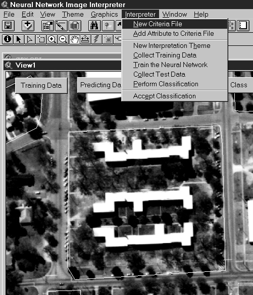¹ The Image Resolution Assessment and Reporting Standards Committee that developed the visible and multispectral NIIRS image rating scale make it clear that spatial resolution (ground resolved distance) is not the only measure of the interpretability of an image. Other factors such as film quality, atmospheric haze, contrast, and noise can reduce the ability of an analyst to detect, distinguish between, and identify objects in an image. See Logicon (1995, 1997), Leachtenauer et al. (1996; 1998), and Pike (1998) for additional information.