GEO 580


LAB 4: Digitizing and metadata

Suggested time for completion: Two weeks


Outline

Purpose
Introduction and background

Data
Procedures Conclusion
What to turn in


4.1 Purpose

In this lab, you will:


4.2 Introduction and background

     In this lab we will be making use of some remotely-sensed imagery.  Hopefully you have been exposed to the basics; if you are completely new to the topic you may want to review some of the web pages listed in the Brief Intro to Landsat-7 section..

A Word on Rasters, Images, and Grids

     In the context of ArcInfo, the words raster and grid are often used interchangeably.  In some contexts, such as ArcToolbox, "grid" refers to a raster in ArcInfo format (there are dozens of methods and formats for storing raster data).

     Digital images are always rasters.  However, not all rasters are images, as we will see when we look at elevation data in Lab 6.  ArcInfo8 can support and display many different image formats, but often times certain tools will only work on ArcInfo's native raster format, the grid.  ArcToolbox can convert many different image formats to grid format, however.  Digital imagery can either be derived from scanned photos, or from airborne or spaceborn electronic sensors.  We will be using data from the new satellite Landsat-7 ETM.
 

A Brief Intro to Landsat-7
More on Landsat 7 & Remote Sensing:

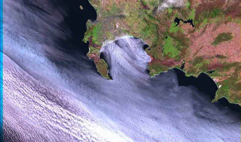
     The first Landsat satellite was launched in 1972.  The first five Landsat satellites carried the Multi-Spectral Scanner (MSS), which recorded light reflected from the Earth's surface in 4 bands of the electromagnetic spectrum.  The resolution was ~80 m.  Landsat 4 and 5 also carried the Thematic Mapper sensor, with a resolution of ~30 m for 7 bands.  Landsat 5 was launched in 1984 and is amazingly still operating. Landsat 6 was lost after launch in 1993.  Landsat 7 was launched on April 15, 1999 with the Enhanced Thematic Mapper plus (ETM+) sensor.  As a result of this combination of foresight and luck, the product of the Landsat program is an invaluable 25-year record of the Earth's surface with high spatial and temporal resolution.  This record is being used to study land-use/land-cover change (and other topics) all around the world.  The liberalized data policy for Landsat 7 will doubtlessly further encourage this research.

Example: North half of a Landsat 7 scene showing Cape Town and the Cape of Good Hope, South Africa.  From the Landsat 7 Home Page.

Cape of Good Hope and Cape Town, South Africa, January 21, 2000.

Basic characteristics of MSS and TM:

     Each pixel of a Landsat image raster contains a brightness value for each wavelength band.  The brightness value, or digital number (DN), is a number between 0 and 255 that is proportional to the number of photons detected by the sensor.  This includes light reflected from the surface as well as light scattered by atmospheric haze and light scattered by the atmosphere itself (the sky is blue because blue light is scattered by the atmosphere; some of this blue scattering is detected by the satellite as well).  It is important to remember that DNs are not just abstract numbers; they represent actual physical measurements of the light reaching the Landsat sensor: sunlight that was reflected by the earth's surface and the atmosphere above it.

     Different materials reflect and absorb different wavelengths of light differently.  For example, chlorophyll in plants absorbs red and blue light but reflects green, therefore plants are green.  Plant leaves reflect very strongly in the near-infrared (NIR) -- if you could see in the NIR, plant leaves would probably appear bright white.  This strong reflectance is exploited in remote sensing to differentiate vegetation and to monitor seasonal and inter-annual vegetation change.  Soils tend to reflect more strongly in the middle-infrared.  Rough surfaces will tend to be darker than smooth surfaces due to increased shadowing.

     The wavelength bands detected by Landsat are listed below (source: AGI GIS Dictionary):

     The ETM+ sensor is similar to TM (Thematic Mapper), except that it adds a second thermal infrared band (band 6b)and a panchromatic band (wavelength 520-900 nm) with a resolution of 15m.  It also has improvements in other areas such as georegistration.

     The thermal band(s) -- band 6 in TM, bands 6a & 6b in ETM -- are usually excluded from land-cover mapping projects.  As you can see, the wavelength of band 6 is much longer than for the other ETM bands; this region of the electromagnetic spectrum is highly sensitive to atmospheric conditions such as water vapor; also, the resolution of band 6 is much coarser (~120 m).  For these reasons, band 6 is therefore usually not very useful for land-cover mapping.  For added confusion, however, band 7 is often referred to as band 6, as it is the sixth band when the thermal bands are excluded.

     The Landsat satellite operates in sun-synchronous orbit, allowing it to cross the equator at approximately 10 a.m. every day.  It repeats a fly over of a given location every 16 days.  Thus the same region can be imaged repeatedly under similar lighting conditions and at high resolution (~30 m for Landsat TM and ETM+, and ~80 m for MSS).  This data has proven highly valuable for vegetation and land-use classification, the study of sediment plumes in rivers and oceans, and the monitoring of land-use change (such as tropical deforestation).


Basic information on orthophotos

Orthophotos are aerial photographs that have been orthorectified -- that is, they have been geometrically corrected so that ground locations are in their true positions on the image and any given area on the photo equals a proportional area on the ground.  Artifacts that need to be removed can be caused by topography (the ground being closer to the plane than usual), variations in the flight of the plane (either in elevation or the tilt of the plane or camera), and by the edges of the photo being more "spread out" and representing more area than the center
.
USGS DOQ Details: DOQ Availability:

     Correcting raw photos is computationally intensive, but a well corrected, georeferenced orthophoto can be highly valuable as a basemap.  GDT, for examples, uses orthophotos to check and correct their street locations.

     The federal government's National Aerial Photography Program (NAPP) has supervised the collection of standardized airphotos covering the entire 48 states, plus Hawaii, since the 1980s.  These serve as data sources for updating the USGS quadmaps as well as for the National Digital Orthophoto Program (NDOP).

     The USGS orthophotos are generally referred to as DOQs (Digital Orthophoto Quadrangles, or Digital Orthoquads for short) or DOQQs (Digital Orthophoto Quarter-Quadrangles).  One would think that 'DOQQ' would refer to the individual orthophoto taken of a single quarter-quadrangle, while DOQ would refer to the area of an entire quadrangle.  However, the USGS DOQ dataset-level metadata page uses the terms interchangeably.

Metadata
More on Metadata

     Metadata is data about data.  You have probably all had the experience of digging through a list of files on a disk one by one because you can't remember the name of the file you want.  You may have had a similar experience working with geographic files; after converting, processing, merging, and editing your data, it is difficult to remember what changes you have made, and which version of your file you wish to use.  Now that geographic data is being made available on the internet on a massive scale, metadata has become the key that GIS professionals and the public will use to find the data they need.

     Furthermore, GIS professionals will often be publishing their datasets and maps, for sale by a company or for distribution to the public.  Publishing the metadata along with the data, in a standardized format accessible to online search engines, will be crucial to help other people find your data, to understand exactly what it contains, and to know the purpose for which the dataset was created.


Metadata standards in ArcInfo8

     The Federal Geographic Data Committee, whose goal is to promote "the coordinated use, sharing, and dissemination of geospatial data on a national basis," has released a metadata standard called the Content Standard for Digital Geospatial Metadata, or CSDGM.  ESRI has a metadata standard as well that is interconvertable with CSDGM.


The Future of Metadata
More on Internet GIS


4.3 Data

The data you will use for this lab includes:

Copy the data to your local work folder.

4.4 Procedures

     Copy the lab 4 data into your working directory.  First we will explore the Landsat image.  If this is your first exposure to satellite images, you needn't worry as none of the tasks will be particularly difficult.  However, you should make sure you understand the introduction above, and don't be afraid to ask questions of your TA or of other students who have taken remote sensing classes.

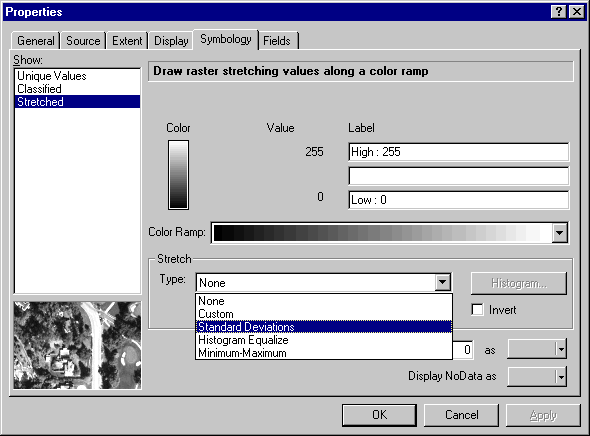
4.4.1 Displaying image data
 

Preview Individual Bands
  • Start ArcCatalog and navigate to your lab4 directory. Notice the available data. 
  • Display the individual ETM bands 1-6, and the panchromatic band in the ArcCatalog preview. 
  • Note: If the images are too dark, follow the next steps and then explore the images.
  • Now view sbetm.tif in the ArcCatalog preview. 
    • View the properties of the image. Also take a look at the metadata attributes.
    • Start ArcMap. Drag sbetm.tif from the ArcCatalog tree into ArcMap.  Note how the sbetm.tif is represented in the ArcMap on the map legend (the left window of ArcMap). 
    • Double-click sbetm.tif in the legend to go to Properties-->Symbology and change the stretch type to Standard Deviations:


  • Examine the "stretched" image.  Image stretching helps, doesn't it?  We will explore this further in a bit, below.
  • Use the same procedure for sbetm-pan.tif, if necessary.
  • Now that your images are stretched, zoom in to the UCSB/Isla Vista area. Note which features appear to be dark and which appear to be light in each band.  While you are doing this, you may wish to display the properties of each TM band - to do this, add the bands individually to your ArcMap project.  In ArcMap you can view the attribute tables. Pay attention to the statistics when comparing the bands. 

 
Question #1: How many pixels are found in each image?  How did you find out?  Why does each band have a different number of records in its attribute table?  What do the attributes "value" and "count" refer to?  (if you aren't able to view the tables in ArcCatalog, try adding the bands individually into ArcMap and viewing the attribute tables)

 
Resampling
  • In ArcMap go to the Properties-->Display tab and change 'Resample during display using:' to Nearest Neighbor.  You will probably have to zoom in to see the differences.  Pay attention to how the image changes appearance. Try all the resample options several times to get a feel for what they do.

 
Question #2: A) Which resampling method looks best for general display?  Which best shows you the original data and therefore is best for analysis purposes? 

B) Change the display method back to RGB Composite.  Which bands are initially represented by which color? What objects/features appear red, green, blue? Why? What objects appear black, white, gray? Why?


Color Stretching

     DNs for each band range between 0-255.  There are a variety of ways to stretch certain parts of this range, to increase the contrast of certain parts of the image.  The "best" stretch will depend upon the analyst's goals.  For example, someone examining sediment in the ocean might stretch just the lowest DNs, bringing out the subtle differences in water brightness

  • Right-click on the sbetm.tif and bring up the Propertieswindow again. 
  • Go to the Symbology tab and change the stretch type from 'Standard Deviations' to 'Histogram Equalization'.  View the results.
  • Change the stretch type to 'Min-Max'. Again, pay attention to how different stretch methods affect the appearance of the image.
  • Go to Properties --> Symbology again and press the Histograms button. View the histograms for all three bands of the RGB composite.
  • Set the stretch type to 'Standard Deviations'. 
     Experiment with the stretch methods and the n (number) for the Standard Deviations setting. Try checking the invert box just to see what it does.  Feel free to experiment with the stretching as you work through the rest of the lab. 

 
Color Composites
  • Go to Properties -- > Symbology again and change the band combination to:  
    • Red = 3, Green = 2, Blue = 1 
      (Referred to as RGB: 321, or 321 for short)
  • Change the combination to RGB:432 and examine the result. 
  • Try 543.
  • Try 654, or any others that occur to you.
     You should decide which resampling/stretch/band combination will work best for mapping features and for distinguishing land-use patterns.  Use this combination when you start digitizing, below.  You may find that different combinations work better for different features.

 
Question #3: A) Which color combination most closely resembles "natural" color (i.e., what you might expect to see in a color air-photo)?  Which combination highlights urban areas, roads, and soils well?  Which brings out vegetation?  For the latter combination, what are the colors of  golf courses, chaparral, dry grassland, and riparian vegetation, respectively?  What accounts for the differences between these vegetation types? 

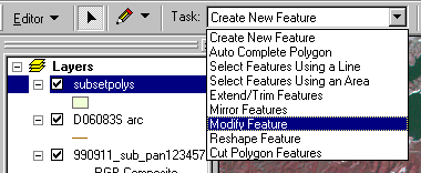
4.4.2 Creation of Line and Polygon Themes from a TM Image
 

     We will digitize new vector themes in ArcMap with the sbetm image as our guide. We will use the new geodatabase data model instead of the coverage or shapefile model.  First, we will digitize a small feature: the shoreline of Campus Lagoon.
Creating a Vector (Polygon) Theme in a Personal Geodatabase
  • If you have any problems creating, and digitizing within a geodatabase, please use alternate instructions found below.
  • Highlight your lab4 folder in the ArcCatalog tree. Go to File --> New --> Personal Geodatabase. Give the database a simple name (e.g., njmgeodbase). 
    • Right click on the new geodatabase in the tree and go to New --> Feature Dataset.  Name your dataset (example: vectors). 
    • To assign a projection to the dataset, click 
    • In the Spatial Reference Properties window, click 


    • Choose one of the existing coverages, such as blockgroups. This will assign the same projection to our new dataset.  When digitizing, it is important that the new dataset and the coverage (or grid) being used for digitization have the same spatial extent.  If they do not have the same extent, you will have difficulties due to inability to digitize "outside bounds."
      • Note that the projection, coordinate system, and datum are now displayed...
      • Details box shows spatial reference: 
    • Click OK,  and OK again if the Feature Dataset window displays the correct projection information.
  • Right-click on your new dataset vectors and go to New --> Feature Class
    • Provide a name (e.g., lakes). Keep the 'Type' on the default (simple features).  Press Next twice. 
    • Your New Feature Class window should be showing you a table with columns labeled 'Field Name' and 'Data Type.' 
      • Click on Geometry (in the 'Data Type' column and the SHAPE field/row).  In the 'Field Properties' below, make sure the Geometry Type is set to Polygon.
      • Your window should look like this:
    • Let's add a new field.  Click and type in the Field Name column, in the row below "SHAPE".  Call it "lake_name".
    • Leave the data type as "text" and below, set the Field Properties --> Length to 30 (this is the maximum number of characters that can be stored).
    • Press .
  • Now that we've created the Geodatabase, Feature Dataset, and lakes Feature Class, we need to move lakes into ArcMap in order to start editing it.
    • In ArcMap, turn off all the layers except sbetm.tif. Drag the new lakes Feature Dataset from ArcCatalog into ArcMap. Note that nothing new appears because no features yet exist! 
    • Change the appearance of the line symbol so that it will be easy to see on top of the TM image.
      • (Hint: yellow, width 2.0 works well)
  • On the Editor toolbar, select Start Editing: 
  • Again, on the Editor toolbar, select Snapping....  Check the boxes for vertex, edge, and end. Close the Snapping window. 
  • One more time, on the Editor toolbar, select Options.Ö set the snapping tolerance to 3 map pixels.
You will find it difficult to decide where the exact edge of the lagoon is on the TM image.  This is because your 30-m pixels will often contain a mixture of lagoon and shoreline, and thus will be of intermediate color.  Do the best you can when drawing the lagoon edge.
  • Select the pencil tool: 
  • To start drawing, place the cursor (mouse pointer) where you want to start sketching the edge of the lagoon on the map.
  • Make sure you are zoomed in to a relatively large (fine) scale. Use the left mouse button to start the line. Every time you press the left mouse button, a new vertex will be added. A single arc can be made of many vertices. Add as many vertices as are necessary to make the arc represent your feature as it appears in the TM image.
  • The red vertex at the end of the arc is the active vertex. If you right-click on the active vertex you are given a menu that includes options such as deleting the active vertex or finishing the sketch. If you right-click off of the active vertex while still digitizing an arc, a more extensive menu appears, with many digitizing options. Experiment with these options if you want. Make sure to delete unwanted arcs using the Undo button.
  • If you need to pan, zoom in or out while in the process of digitizing, simply click on the tool that you need, e.g., Pan: .  (Unlike ArcView, your sketch will not be lost). Then choose the pencil tool again to continue where you left off.
  • When you are finished digitizing a single arc, you can finish the sketch with either of the right-click menus or you can double-click the left mouse button.
  • When you want to start a new arc, if you are within the snap tolerance of an existing arc (~ 90 meters here) the new arc will automatically be "snapped" to the existing arc.
  • Digitize other water bodies (e.g., Devereaux Slough, Lake Cachuma, etc.) for practice, if you wish.

Alternative Instruction if Geodatabase Can't be used due to Errors
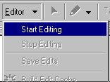
  • If you encounter an error in creating polygons using a geodatabase, where it tells you that you are 'out of bounds', you may not be able to complete the assignment using a geodatabase.  Instead you will need to create a coverage and digitize polygons into the coverage.
  • 1. Right Click in Arc-Catalog -> Create New Coverage (bottom option).  Give it a name, and assign it the projection of Blockgroups.  Next select the feature type as polygon.  Add the fields needed either now or later from ArcCatalog (as you did in lab 3).
  • 2. Add the background image to ArcMap.  Add the new coverage to ArcMap.  Make sure its on top of the image.
  • 3. Click 'Start Editing' (Add the toolbar if missing).  Use 'Add New Feature' to add a bounding polygon to add your bounding polygon. 
  • 4. Add new polygons by using 'Auto Complete Polygon' only!!  This is because a coverage uses continuous model space, and you will not be able to connect polygons together if you use 'add new feature'.
  • 5. Note: You cannot easily undo a polygon you created in a coverage.  Thus, to 'Undo' a mistake, save your edits often, and if you don't like what you created, choose 'Stop Editing' and don't save your results.  Then start editing again, and everything not saved will be gone.
  • You will need to use a coverage later if you encountered this error here where you digitize landuse and highways.

 
Editing Vector Feature Geometry

     Inevitably, you will decide that you want to move some of your vertices.  Unless you want to redraw the whole feature, do this:

  • Go to the Editor tool bar (not the Editor button) and click on the 'Task' menu.  Select 'Modify Feature':
  • Using the Edit tool, click on your lake feature.  The vertices of your polygon will now be displayed.  You can click and drag them to move them.


Giving Your Digitized Feature Name Attributes

     Now that you have digitized the lagoon, you will attribute it with a name. 

  • Right-click on your lakes theme in the ArcMap legend and select Open Attribute Table.  The selected polygon appears blue in the map, while it is also highlighted within the attribute table.
  • Click on the blank lake_name cell. Type in the name (e.g.: Campus Lagoon).
    • Hit Return or click on the next row to finish entering the name.
    • You can select the next polygon to attribute in the table by clicking on the left of the row. 
    • You can also select the polygon you want to attribute on the map by using the Feature Editor tool, .
      • WARNING: This tool can be used to move features. Make sure you do not move the feature after you select it.

 
Saving Edits and Turning Off Edit Mode

     When you are done creating and editing your feature, select Editor --> Save Edits and Editor --> Stop Editing.

4.4.3 The Effect of Resolution on Digitizing

     As you could see when digitizing the lagoon, coarse resolution makes it impossible to draw borders with high precision.  We will digitize the same lagoon using the 15-m panchromatic band from ETM.
 

  • Turn off the other image layers in ArcMap and bring in the panchromatic band (sbetm-pan.tif). 
    • Display it in ArcMap with the default grayscale color scheme. 
    • Make sure the resampling is set to Nearest Neighbor. 
    • Repeat the digitizing of the lagoon (simply create another feature in your lakes feature class, digitizing on top of your first lagoon feature).

 
Answer Question #4: A) Compare the resulting lagoon features.  What are the differences between them?  Account for the differences. 

B) Does the 15-m resolution image contain mixed pixels?  Would you expect mixed pixels in the high-resolution DOQ?  Why or why not?  Is it possible to have an image raster without it containing any mixed pixels?

Note: To answer part B, it may be helpful to look at a wider range of resolutions.  To see what the campus-lagoon region looks like at different resolutions, color composites, etc., check out the various parts of the UCSB Geography 115B lab #1 page.

     Now, digitize Highways 101 and 217 across the whole ETM image.  Use 30 m bands with a useful color arrangement, or the panchromatic band, whichever you prefer. Make sure the arcs are snapped where these roads meet. Add any other roads you want as long as you can identify them 
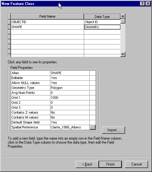
well in the image.  Digitize these as lines, in a new Feature Class named something like etmroads.  Note: You may need to save and close your ArcMap file in order to create the new Feature Class.
 

Digitizing Your Highway Theme

     In order to digitize line features like highways, follow the instructions that we used for lakes.  The only only difference from digitizing a polygon will be to set the Geometry Type to Line while you're in the 'New Feature Class' wizard.

  • When you are done adding the road names, go to Editor --> Stop Editing.  Save your changes (unless you messed up).
  • Display the gdtstreets coverage with your etmroads theme, without the ETM scene in the background.
  • If this doesn't work, you may need to use a coverage instead of a geodatabase, see the instructions above (in this same color).  Remember to create a coverage with the feature class arcs instead of polygons as above.

 
Answer Question # 5: A) How do the two roads datasets (Coverages or geodatabase feature data sets) compare (the one you just created, compared to the one which came with the lab)? Which one has smoother lines? What are some sources for the differences between these two datasets? B) What other attributes might you want to add to your roads theme?

 
Giving Your Digitized Feature Name Attributes

     Now that you have digitized all the roads and water bodies that you want, you will attribute them with names (this is a repeat of the procedure used for Campus Lagoon).

  • Right-click on your roads theme in the ArcMap legend and select Open Attribute Table.  The selected arc appears blue in the map, while it is highlighted in yellow within the attribute table.
  • Click on the blank road_name cell. Type in the name (example: Highway 101).
    • You can select the next arc to attribute in the table by clicking on the left of the row. 
    • You can also select the arc you want to attribute on the map by using the Feature Editor tool, .
      • WARNING: This tool can be used to move features. Make sure you do not move the feature after you select it.


4.4.4 Creating Land-Use/Land-cover Polygon Themes

     We will now create a choropleth map showing broad land-use/land-cover categories for our ETM image.  We will do this by visual inspection; however, the most common method of classifying an image is with a classifying algorithm  that classifies pixels based on the similarity of their spectra to the spectra of training site pixels.


Possible Bug:

Using version 8.1, "autocomplete polygon" will ONLY work if your polygon theme is added before your TM image.  It is unknown if this is also true in previous versions of ArcInfo.


  • You should now be familiar with the steps to create a new Feature Class.  Using the same Feature Dataset as the one we've been using, create a polygon feature class named etm_lulc.  Make sure you give it a 'name' field as well. 
    • Put etm_lulc in ArcMap and double-click on it.  Make the polygon symbol "hollow" with an outline color and width that will show up well against the TM scene. 
    • Once the etm_lulc theme is selected, start editing.  Set the snapping and options as you did for the lagoon theme, except that you can set the tolerance to a larger number (say, six pixels) to make it easier to digitize while zoomed out.
  • The polygon theme should be exhaustive for the whole TM image, in other words, all space occupied by the TM image should end up with classified polygons. The theme should also have correct polygon topology. 
    • We want to digitize polygons that represent various land uses or land covers. Often these are ambiguous, so keep it relatively simple. (These land-use/land-cover classes would be appropriate: ocean, chaparral, agriculture, urban-developed, UCSB, open space/grassland).
    • Since the theme will be exhaustive, the first polygon to digitize will be a "bounding" polygon. This polygon will have one vertex at each corner of the TM image.  Zoom in to place each vertex precisely.
  • The next polygon to digitize will be the ocean. Now that we have the "bounding" polygon, we essentially need to just digitize the coastline. That will split the "bounding" polygon into two polygons. However, if we use the normal polygon drawing tool, this will duplicate the arcs of the "bounding" polygon, which would lead to sliver polygons wherever the arcs do not match up exactly. So, we will use a slightly different method. 
    • On the Editor tool bar, set the 'Task' to Auto Complete Polygon. Now we will digitize the coastline. The software will create the polygons automatically. However, it will work ONLY IF both end vertices are snapped to the existing "bounding" polygon. So make sure you start the new arc no more than 3 pixels from the "bound".  Zoom in to ensure that it is snapping. Can you see the circle snapping to the feature?
    • When you have digitized the last vertex, make sure it has snapped again to the "bound". To finish the polygon, double-click the on the last vertex. (Or right-click and select the 'Finish Sketch' option).  If both ends are not snapped, the line will disappear and you will need to start over.  Zooming in is the best way to ensure that you don't lose your line when you double-click. 
  • Using the auto complete polygon task tool, digitize 10-20 new polygons that distinguish varying land uses or land covers. 
  • When you're done digitizing you will want to attribute each polygon. Open the table, select a polygon, give it a name attribute. Name each polygon land-use/land-cover class.
  • When you're finished, stop editing and save changes.
  • If you cannot create polygons because of the error 'out of bounds', you will need to create a coverage instead of using a geodatabase.  Follow the instructions given above (in this same color).  Other than using a coverage, you will still need to follow these directions too.  Its the same, other than its harder to erase mistake polygons.

 
Answer Question #6: A) Describe the decision-making process you used to determine land-use/land-cover boundaries. What qualities in the TM image helped you define the boundaries? B) How could you quantify the accuracy of your land- cover classes or boundaries? How was error potentially introduced into your land cover theme?

4.4.5 Creating a Map Overlaying LU/LC Themes on Image

     Now, you are going to create and print a map showing the themes you created on top of the ETM image.  While designing your map keep in mind your goals: you want to convey a sense of the the topography and clearly show your LU/LC classes, along with your road theme.
 

Displaying Themes on Top of Satellite Image
     For your etm_lulc theme, 
  • Go to Properties --> Symbology --> Categories --> Unique Values --> Many. Make the feature name the value field. Then click Add All Values. 
    • Change the color of each unique polygon in the legend. Use intuitive colors such as green for vegetation, dark blue for ocean, etc. 
    • Set the outline to none for a cartographic effect.
  • Double-click the new land use theme in the legend. Go to Display and set the % Transparency to 50. This will allow you to see the TM scene beneath your land-cover choropleth.  You can experiment with this value to find what you like best. 
  • Right-click on the new land use theme and select Label Features.
     For your roads theme,
  • Add your new roads theme to the map. Change the line symbols using Symbology --> Categories --> Unique Values.  Label the roads.

 
Your map for Lab 4: Finish the map using the layout environment of ArcMap. Add a title, north arrow, legend, scale-bar, map cartographer (that would be you, the author), date, and a brief text description (a sentence or two) of the data sources (review the introduction). 

*** Although you will print the map on a grayscale printer, focus on making a good color map. Color is an extremely effective tool, especially when working with rich data such as Landsat TM, and multiple themes.***

4.4.6 Metadata Display and Editing in ArcInfo8

     ArcCatalog contains a metadata editor that allows the user to easily view metadata about a dataset's contents, attributes, and spatial referencing.  The editor also allows metadata entry, conversion of metadata between formats, and the attachment of additional files to a metadata file.  A number of optional settings allow the user to decide if metadata standards will be enforced (i.e., must all of the required fields be filled in before the data is used (??), and if the metadata changes will be "logged"; that is, will changes made to the data be recorded, creating a history for the dataset.

eXtended Markup Language

     ArcInfo8 stores metadata in XML format.  XML stands for eXtensible Markup Language, which is similar to HTML (Hypertext Markup Language) used for webpages.  It is a standardized, open language designed for exchange of structured documents on the web. http://www.xml-zone.com/ defines the difference between XML and HTML thus:

"While HTML specifies how a document should be displayed, it does not describe what kind of information the document contains, or how it's organized. XML fills this void and allows document authors to organize information in a standard way."
     If a geographic dataset does not already have metadata, ArcCatalog creates an XML file for it.  The XML format makes the metadata easily searchable.  Older metadata found on the web is often in HTML format.  We will explore some well-structured HTML metadata in addition to the XML capabilities of ArcInfo8.
Metadata Content
     The main types of information necessary for geographic metadata are described below (Summaries are from, and links are to, the Metadata Education Project at the UWyo Spatial Data and Visualization Center):
Identification Information: description, purpose, creator of the dataset and the area and time period it covers
Data Quality Information: sources, processes, accuracy statements
Spatial Organization Information: the data model used (internal structure of the data)
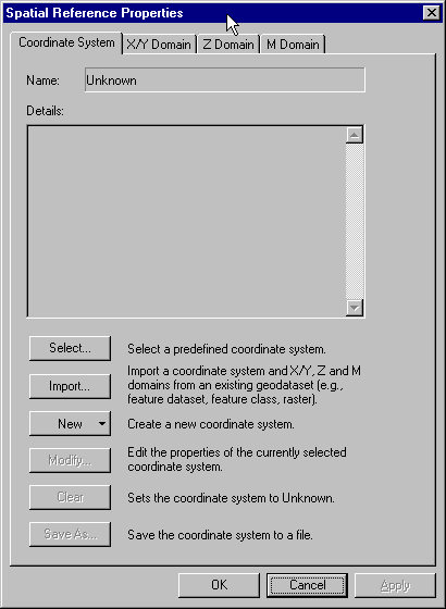
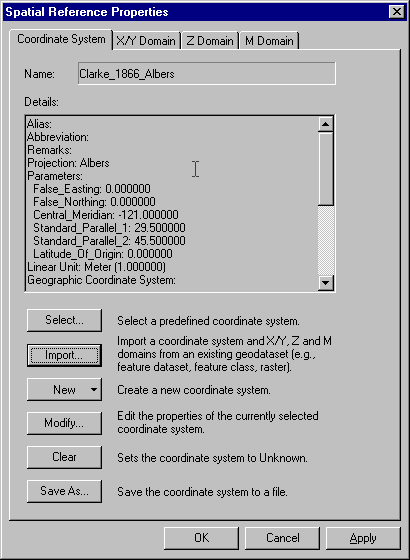
Spatial Reference Information: coordinate system/projection and datum
Entity and Attribute Information: details on what the dataset describes
Distribution Information: where/how to get the dataset
Metadata Reference Information: who wrote the metadata and what version it is
Metadata in HTML format
     Having a GIS-integrated program such as ArcCatalog as a metadata creator and viewer is a relatively new phenomenon.  Much of the metadata you will encounter is published in HTML format on the web, created by programs such as mp. mp stands for Metadata Parser, a program that converts an indented ASCII metadata file into formats such as HTML, text, or FAQ format (for display on the web), or formats such as SGML or XML (for search in a data clearinghouse).

     To familiarize yourself with metadata content and layout, examine the metadata for the LANDCOV layer found on the California Gap Analysis Project Webpage (hosted by the UCSB Biogeography Lab).  You do not need to download the data from the website, as we have already clipped it and put it on the network for you.  You will go to the webpage to look at the metadata, however.  We will be using a subset of this data layer for part of Lab 6.  Answer these questions:


Answer Question #7: A) What extra elements in addition to the seven standard elements are listed in the LANDCOV metadata? 

B) Briefly describe (1 sentence) the LANDCOV layer.

C) What is the MMU (minimum mapping unit) for the dataset?

D) What was the main data source upon which the polygon boundaries were based?

E) What projection and spheroid are the data in?


ArcCatalog Metadata Editor
     You are already familiar with viewing metadata in ArcCatalog.  You will now learn how to create metadata, convert metadata between display styles and formats, attach metadata files, and attach additional metadata.
 

Creating Metadata Using the ArcCatalog Metadata Editor

     You are already familiar with ArcCatalog's metadata tab: .  Look at the metadata for your etm_lulc theme.  It should already have spatial reference information. 

  • This is the Metadata Tool Bar: .
  • To edit your metadata, Click .
    • This brings up the Metadata Editor:
  • Fill in the all of the REQUIRED metadata fields for all of the headings and tabs. 
    • Put unknown or not applicable (N/A) if necessary for some fields. 
    • Save your changes and return to view your metadata.


Viewing Metadata via Stylesheets

     The metadata you have created was saved in XML format.  This allows the information to be displayed in multiple ways.

  • Change the Stylesheet to see the XML code.  The tags you see identify the text blocks as specifying particular kinds of information.  Whereas in HTML, a tag modifies the display of the text (e.g., <B> starts boldface type), in XML the tag says what the text refers to (e.g., <descript> denotes the beginning of the data description).
  • View the metadata with the FAQ stylesheet. 
  • View the metadata with the FGDC stylesheet.  This format should look familiar to you from the California Gap Analysis page.
Importing/Exporting Metadata
  • Click to import metadata.  This might save you a lot of typing when using a new dataset sometime in the future.  Note the formats that you can export metadata to.
  • Click  to export metadata.  Note the formats that you can export to.
Metadata Properties
  • Click , then go to the Options tab to change your metadata properties for this layer.  The only option is a toggle to turn off automatic metadata update.  Don't change this.

 
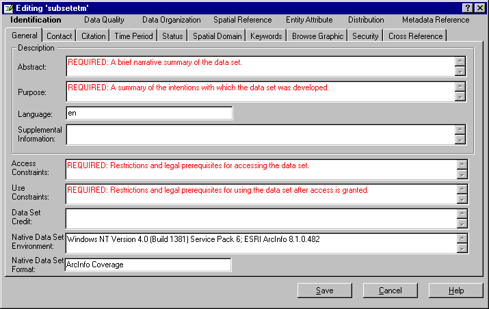
Answer Question #8: A) What are the main differences between the stylesheets?  Which do you prefer, and why? 

B) What formats can you import metadata from?  What formats can you export metadata to?


Print out your metadata in the FGDC stylesheet and attach it to your lab.


4.5 Conclusion

     In this lab, you have been learned how to digitize features on-screen.  Often digitizing is also done directly off of paper maps, but that procedure is better covered in a cartography class.  You have also been exposed to some of the most common imagery used for digitizing and land-use/land-cover.  You now know how to alter raster display to improve digitizing and to gather more information from your image.

     You have learned how to view, read, create, convert, and search metadata.  While metadata creation is often considered tedious and expensive, remember that metadata is the key that allows you, as a data producer, to make your data available to the world GIS community.  It also gives you, as a GIS user, the ability to find useful spatial data in the free-for-all of the World Wide Web.


4.6 To turn in


Lab originally created by Nicholas Matzke and Sarah Battersby
UC Santa Barbara, Department of Geography
© 2000, Regents of the University of California; redistributed by permission

Last update: April 25, 2002
http://dusk.geo.orst.edu/buffgis/Arc8Labs/lab4/lab4.html