Lab 2: GIS Data Models and Data Structures
Instructions below updated for ArcGIS 9.3
Click here for ArcGIS 9.1/9.2 version
Suggested time for completion: One week
Outline
2.1 Purpose
To gain a clear understanding of what a data model is, and why data models
are important.
To learn the data models and data structures that ESRI supports in ArcGIS 9,
and the similarities and differences between them.
To learn the advantages and disadvantages of using certain data structures
for different tasks.
To reinforce basic ArcGIS 9 skills.
2.2 Introduction and
background
For more information on data models in Geography:
You will notice some diversity in the definitions, as they
are in the context of different companies, software, times, and degrees
of specificity. For this lab, focus on the hierarchy
described in the main body of the lab and in GEO 580 Lecture #3 in class.
Data models in geography:
AGI dictionary Definition
of "Data Model" (their server may be down though)
ESRI GIS Dictionary Definition
|
Geographic Data Modeling: An Introduction
Data models are a crucial concept for GIS users
to understand. Data models describe how geographic data will be represented
and stored. The choice of data model will yield benefits in terms of simplifying
aspects of the real world, but will also incur costs in terms of oversimplifying
or misrepresenting other features.
A map is an example of an analogue data model(
1); the cartographer has abstracted the real world with a set of conventions
that she can use to represent important aspects of the landscape. In a
computer, all information must be stored digitally: that is, it ultimately must
be reduced to numbers (1010000110...). Therefore, the abstractions of
a real-world model must be formalized in a data model. The data
model shows the computer how best to store the geographic information (geometry
and attributes) in a database or other format. Bernhardsen (1999) diagrams
the process along these lines:
Figure 1: The modeling process. The real world is described by the data model. The "database" is part of the resulting data structure (how the data model gets implemented in a digital computer).
(after Bernhardsen 1999, p.39. Bernhardsen, Tor. Geographic Information Systems: An Introduction. New York: John Wiley & Sons, Inc., 1999, pp. 37-99.
Graphic from www.gis.com)
In order for geographic data to be represented digitally,
a geographic data model has to be chosen. Most of the confusion
about data models arises from the diversity of geographic data models.
Unlike classifications of things in the natural sciences or geometry, data models
are not necessarily defined by hard-and-fast rules derived from observation
or logic; data models are instead created by GIS programmers and users for the
purpose of representing certain specific features from the real world.
The definitions and capabilities of data models will thus vary depending upon
the aspect of reality that the GIS software designers and users are attempting
to model. Furthermore, data models (and the resulting data structures
that are actually implemented in GIS software) may evolve through time under
the influences of technology (e.g., increasing storage space and processing
power, or networking, or software compatibility) or even history (e.g., ESRI
started with the georelational model way back in 1980, so it is still probably
their best-supported and most used data model). Finally, the influences of the
marketplace and the interests of GIS companies and consumers must be taken into
account.
The result of all this is that every GIS software package
will be capable of supporting a number of data models. The capabilities
of the data models may change with new versions of the software, and compatibility
issues may arise. Certain functions will be accessible with data in the
form of one data model but not another.
Data Models vs. Data Structures
A data model is a conceptual model of the real world. The representation
of this model in the computer is the data structure . A given
vector data model could be implemented in a computer in a number of ways.
In practice, however, the software designer has usually done both the data modeling
and data structuring, so that when one refers to a "coverage" both the data model
and data structure are pre-defined. This is not necessarily the case with custom
user-designed data models, however.
The data structure therefore corresponds to the fourth
box, labeled 'DATABASE,' in Figure 1: The Modeling Process
.
The confusion surrounding all of this can be reduced
if one thinks of the data models as fitting within a general hierarchy (these
will all be discussed in detail in lecture).
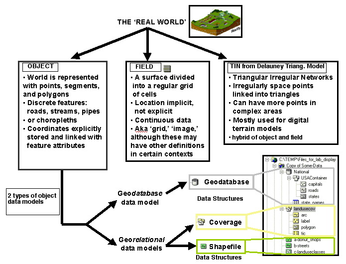
Figure 2: Hierarchy of ESRI's data models and data structures.
. Beware, as ESRI documentation often uses the same names for both data model and data structure, which may be confusing (e.g., ESRI's geodatabase data model and geodatabase data structure. ESRI also developed a "georelational" data model which they sometimes call the "coverage" data model as well. And the resulting data structure is also the "coverage", i.e., the ArcInfo coverage). TIN is a
data structure resulting from the Delauney triangulation data model.
One final complication is that geodatabase data structures
(based on ESRI's object-oriented geodatabase data model) may contain rasters
and TINs, as well as vector data sets.
Data Models, Data Structures, and
Feature Classes in ArcGIS 9.
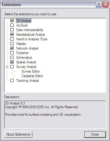
In ArcCatalog, the geometry and data structure of every
feature is identified by a small picture or icon. This works much
like Windows Explorer, except that only file formats recognized by ArcCatalog
as geographic data will be displayed.
Your life will be made much easier if, as part of learning
about data structures, features, and other files, you learn ArcCatalog's icons
for them. There are a lot of them and they can be initially confusing,
so here is the handy table from Lab #1 that you can refer back to. Below is a display from ArcCatalog
showing how the icons are identified by type.
|
Also, you can also always click on the 'Contents'
tab while highlighting the folder above the file in question., like
this:
|
 |
The folders and files that make up shapefiles, coverages,
geodatabase feature classes, rasters, and TINs fall into an organizational hierarchy
in ArcCatalog (Note: this is a completely different matter than the
conceptual hierarchy discussed above in Figure2). Figure 3 below
shows the hierarchy of folders, data models, data sets, and feature classes
as displayed in ArcCatalog. Feature classes are the lowest level that
the user accesses.
- For shapefiles, the shapefile is the feature class. Each
feature (donut shops, streets, etc.) will be contained in its own shapefile.
The geometric information (ArcCatalog 'hides' these binary files, but in
windows explorer they are seperate files- DONT USE WINDOWS TO MANAGE YOUR
DATA) will be displayed in the "Geography Preview" and the attribute information
(stored in dBASE IV tables) will be displayed in the "Table Preview".
This linkage of geometric files to separate attribute tables is common to
shapefiles and coverages and is the main conceptual tenet of ESRI's georelational
data model.
 |
Figure 3: ESRI icons and hierarchy. |
- For coverages, each feature class does not correspond
to a map feature. The coverage feature classes are standard categories
like arc, label, polygon, tic, etc. The feature classes are found
in a folder. This folder is the coverage. Each
feature on the map (landuse, railroads, etc.) will correspond to one of
these coverage folders. Within the folder, the feature classes store
the geometric information (coordinates are stored in hidden binary ARC files;
displayed in the "Geography Preview") that is linked to attribute tables
(INFO tables; displayed in the "Table Preview"). Like shapefiles,
coverages are data structures resulting from a georelational data model.
- For geodatabases, like shapefiles, each feature class corresponds
to a map feature such as roads, counties, etc. The feature classes
are generally grouped into a feature data set, a folder that might
contain data about a region or topic (e.g., "USA container" contains information
about the USA). Unlike shapefiles and coverages, geodatabases employ
a geodatabase data model that stores each feature as a row in a relational
database table (this record would link to other tables containing geometric
information, topological relationships, attribute information, etc.).
A number of feature data sets can be stored in a geodatabase.
- Looking again at Figure 3, you will notice that the geodatabase, the
coverages, and the shapefiles are all contained within the the folder 'Some-Data.'
The little blue symbol on the folder indicates that it contains recognizable
geographic data in the first level beneath 'Some-Data.' In the context
of coverages, this folder would often be referred to as a coverage workspace.
- Additional note:
Notice that we did not name the folder "Some-Data"
as "Some Data" - with a real space - even though this is allowed by
Windows. ArcToolbox needs to read directory path names into a command line
to run certain commands, and if there is a real space in the file name,
the path will be split and interpreted as two separate words. You will get
an error such as "Spaces are not permitted in the path name"
or "too many commands" or some such. So, for ArcGIS
purposes, name your directories and files using dashes ("-") or underscores
("_") instead of using spaces. Also try to keep all names under 13
characters. You have been warned!
2.3 Data
mystery -- Folder containing 8 data layers of several features in
different data models. You will be figuring out what these are in the
lab.
roads -- multnomah county roads coverage
mult_dem -- digital elevation model of Multnomah
county
mult_tin -- TIN derived from mult_dem
mult_cont -- Contour shapefile derived from mult_dem
or_counties -- counties of Oregon, from the
Oregon Geospatial Data Clearinghouse
Download the data here (36 Mb) into your local work folder.
2.4 Procedures
2.4.1 Understanding data models: Tables
Question 1:
As you work through the lab, fill out Tables A and B in the word
document that you will be turning in, based on information from the lab introduction,
exercises, course text, and lecture. If time is short, you may want
to leave some of the tables to fill out outside of class. |
Table A: Main Data Models. Briefly describe each data model.
| Geographic Data Model |
Object
|
Field
|
Delauney Triangulation
(hint: for TIN data structure)
|
| Briefly describe the essential characteristics of each data model.
Include the types of data generally represented by a particular data model
(i.e., continuous or discontinuous) and the data structures that would be
implemented in GIS software by the data model. Give an example of
a likely geographic feature that would be represented by each model. |
|
|
|
Table B: ArcGIS 9 Vector Data Structures.
| Fill out the table as you work through the lab. If you need additional
information, make sure you examine lecture notes, reading for the course
(Zeiller's "Modeling our World"), and the ArcGIS help files. |
Table B:
Fill out Table B in your lab2questions_93.doc file |
ArcGIS Help
ArcGIS Help works like any Windows program help
section.
- Go to the Menu Bar --> Help --> ArcGIS Help:
- When you're looking for something in ArcGIS Help, make sure to
Search in both the Index and the Search tab. Trying the search
with different terms (e.g., data models, or coverage, or geodatabase)
increases the odds of finding something useful.
- Also, for more information you can check out the Getting more
help section, especially Using this Help system and ArcOnline:
|
2.4.2
Mystery Models
Examine the layers in the 'mystery' folder using ArcCatalog
or ArcMap.
Answer question 2:
What are the data models and data structures for each of the layers? What feature does each layer represent? (be as specific as possible).
mystery1 --
mystery2 --
mystery3 --
mystery4 --
mystery5 --
mystery6 --
mystery7 --
mystery8 --
|
Once you have identified the layers and the conceptual data
models that they are based on, convert mystery5 into the same
data structure as mystery7. You will have to figure out how to do this
yourself, but here are some big hints:
Converting
Between Data Structures Based on the Data Models
- You will have to use ArcToolbox to accomplish this task.
Recall that you can open ArcToolbox from the Start menu or by clicking
on the ArcToolbox button (
 )in ArcCatalog.
- We are doing a conversion, so navigate to the toolbox menu that
would contain the appropriate tools.
- Find the appropriate sub menu for converting data in mystery5's
datamodel.
- Find the tool that will let you convert to mystery7 's
data structure.
- You should be able to figure out which layer to use as input.
Recall that you can drag-and-drop from ArcCatalog instead of typing
or browsing. Use the defaults for everything else unless you are in
an experimental mood.
- Did this work??? If you got an error (you should have), it has to
do with the functionality of ArcToolbox. This particular conversion
requires an integer Grid - This Grid is floating point. You will need
to convert the grid to an integer before you convert it to the new
data structure. How to do this:
|
Give the output a name you will remember, and run the conversion.
Take your resulting layer and display it in ArcMap, along with mystery5.
Answer question 3:
How similar are mystery5 and your converted layer? Briefly
describe the major differences between the two. What is the cause
of them? What do you think was the source data from which mystery5
was derived? |
Go to the data directory lab2_data.
Now, add mult_cont, mult_dem, and mult_tin into
ArcMap. Display just mult_cont and mult_tin, and overlay mult_cont
on top of mult_tin. To make the display intelligible, you will
have to change the properties for the two layers.
| Changing Layer
Properties in ArcMap
To change the Properties of a layer
(let's use mult_tin) in ArcMap, right-click on it in the
legend and go to Properties (Double-clicking also works).
You should be familiar with the Properties window from Lab 1.
- You get a large window with many tabs, like this:
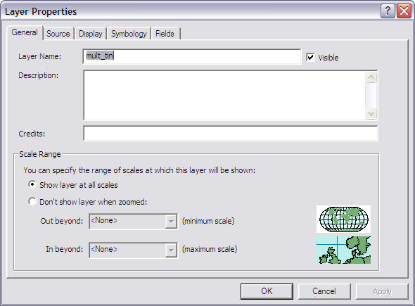
- Go to the Display tab.
- Change the transparency of mult_tin so that the DEM raster can be
seen underneath it, and hit OK.
- Make sure the mult_tin layer displays on top of the DEM
raster.
|
| If you're curious about making better
use of Properties, the main methods are the creation of Layers in ArcCatalog,
and ArcMap's Style Manager, found in the Menu Bar under Tools-->Styles-->Style
Manager. |
You will be repeating these steps to change
a layer's properties hundreds of times throughout the quarter. You
will probably find the Properties functions very useful but perhaps not
as user-friendly as they could be and somewhat tedious and frustrating
to use for complicated tasks. We will discuss ways to make this
easier later on in the quarter by using ArcMap's Style Manager. |
Answer question 4:
Which of the three layers (mult_dem, mult_tin, mult_cont)
do you think was the original data layer? Which is "second generation"
and which is "third generation"? Why do you think this? |
2.4.3
Data Structures and ArcToolbox
Coverages are the vector data structures long used
in the old Unix workstation version of ARC/INFO. Therefore, many of the
ArcToolbox tools simply use a wizard to create a command line that runs an ARC
process in the background. As a result, many of the tools only support
coverages, although some of the newer tools are designed for geodatabases or
shapefiles. To familiarize yourself with the Toolbox and the input formats
required, find each tool listed below and figure out what kind of input file(s)
it supports (e.g., coverage, geodatabase feature class, grid, TIN, etc.).
Finding and Examining Tools
- Again, recall that you can open ArcToolbox from the Start menu
or by clicking on the ArcToolbox button (
)in ArcCatalog.
- If you can't find a particular tool in ArcToolbox, try the Search
tab --> Locate and search by name or description.
- For more information on a tool, right-click on it and click Help.
|
Answer question 5:
Find each of these tools and determine what data structures (or perhaps
other file types) it takes as input:
a) Clip, Select, Intersect, Buffer, & most other Analysis Tools
(all the same answer)
b) Import from SDTS (in Conversion --> To Coverage)
c) Feature Class to Geodatabase
d) Export to Interchange File
e) Join Info Tables
f) Labeling Polygons (create labels)
|
2.4.4
AATs and PATs
As discussed above, coverages have been the standard
data structure for the generic vector data model for previous releases of Arc/INFO.
With the release of ArcGIS 9.x, Arc and INFO have apparently been integrated (with INFO essentially replaced by MS Access tables),
and the new geodatabase data structure has been promoted. However, coverages
are still a very commonly used, and it therefore behooves us
to understand their structure.
Recall that coverages are based on the georelational
data model. The INFO part of Arc/INFO was a relational database manager.
An INFO file is a table that stores the information associated with the geographic
features of a spatially referenced data set. This gives a GIS the ability to
manipulate information both spatially and via standard tabular database functions.
An example relational model is when two tables share a common column. In a georelational
model the individual records in two or more tables are related through their
location in space. The polygon coverage below serves as a simple example of
this concept. The common column is often called the KEY column and is used for
relating or joining tables.
(courtesy of ESRI)
Let's explore the attribute tables of roads.
Go to ArcCatalog and Preview the data.
Previewing Tables
- Below the preview map, locate the Preview box:
 .
.
- Change the preview option from Geography to Table
.
- You are now looking at the arc attribute table (AAT).
Answer the question below. |
Answer question 6:
How many records are there? What do FNODE# and TNODE# mean? What
other attribute information can you recognize or guess at in the table
(pick 3 columns)? |
For a look at polygons and Polygon Attribute Tables
(PATs), open mult_county. Explore the tables for the tic, label,
arc, and polygon coverage feature classes.
Sorting
a Column in Table Preview, and Searching for a Text String
- To sort a table (e.g., polygon), for example by name, click
on the column heading you wish to sort.
- This should highlight the column you wish to sort by.
- Then, right-click and select Sort Ascending.
Now open the cacounty coverage, examine the coverage feature classes and
note the differences. What is the region.cty feature class? Now answer
the questions below. |
Answer question 7:
How many counties are there in California? Why do the AAT, PAT,
and RAT have different numbers of records? Explain the relationship
between arc, and polygon featue classes in this coverage.
What are the label and tic feature classes for?
Hints: To figure out the answers, you will need to examine
the tables. In addition, you might want to use the Identify
Tool ( )
in the Geography Preview. Also use ArcGIS Help as
described above. )
in the Geography Preview. Also use ArcGIS Help as
described above.
|
Your map for Lab 2:
Make a map of Multnomah County, Oregon with
the roads coverage overlaid on the contour coverage, using your knowledge
& skills from Labs 1 and 2.
Make sure you follow the basic
principles of cartography outlined in Lab 1. |
2.4.5
Relationships in GIS
So far we have focused on digitally modeling geographic
features, and attributes for those features. However, increasingly GIS
users are increasingly seeking to model relationships between features
as well. These relationships can have behavior and can follow rules.
A primary advantage of the new geodatabase model is that it gives the user/designer
the ability to build structured relationships between features.
To get a handle on this, consider the classic example
of a power pole and a transformer. Perhaps you want to describe the location
of the transformer on the pole -- e.g., height in feet and the side of the pole
the transformer is on (North, West, etc.). The geodatabase designer could
constrain the possible entries in the "location" field for the transformer to
North, South, East, and West. Then, a person doing data entry would simply
select the appropriate direction from the available options. Similarly,
the designer could constrain the "height" field to between 10 and 20 feet.
The designer could also limit the number of relationships
a particular pole can have with transformers. In the real world, several
transformers can reside on a pole. However, an unlimited number of transformers
will not fit -- we might imagine that four transformers is the maximum.
The geodatabase designer could constrain the number of relationships the pole
has with transformers to between 0 and 4. After four transformers have been
assigned to that pole, a transformer would have to be deleted before another
could be added. .
The relationship between poles and transformers is
directional as well. In a directional relationship, changing A
will change B, but changing B will not change A. If you move a pole (in
real life and in the GIS), you want the transformers on the pole to move as
well. But you don't want to be able to move a transformer by itself, as
it must always be on a pole. If you delete a pole from the data layer
(say, because it was burnt down in a forest fire), you will want the records
for the transformers on that pole to be deleted as well. But if you delete a
transformer, the pole should remain unaffected.
Answer question 8:
Come up with an example of two simple (geographic) features that you might
want to represent in a geodatabase as having a relationship. Come up with
some rules for the relationship describing directionality and data entry
constraints. This is just a conceptual exercise, so you do not have
to actually create the relationship rules in the computer. Creativity
is fine for this question as long as you show that you understand the
concept of relationships between features. |
2.5 Conclusion
In this lab, you have gained a basic understanding of geographic
data models and data modeling, and the resulting, primary data structures used
in ESRI's ArcGIS software. You have seen how the ESRI data structures
are similar and different from each other, and how each has advantages and disadvantages
for certain purposes. You have gained further experience with some basic
ArcGIS skills, such as changing properties and using the help functions.
Finally, you have learned about the important concept of relationships in GIS.
2.6 To turn in
- The question sheet, with typed answers (Word document)
- One map of Multnomah County
Lab originally created by Nicholas Matzke and Sarah Battersby
UC Santa Barbara Department of Geography
© Regents of the University of California; redistributed by permission
Modified by Dawn Wright, Jeremiah Knoche, and Tracy Kugler, OSU
http://dusk.geo.orst.edu/buffgis/Arc9Labs/Lab2/lab2.html