Introduction
Arc Marine (or the ArcGIS Marine Data Model - MDM), is a geodatabase model tailored specifically for the marine GIS community. Created by researchers from Oregon State University, Duke University, NOAA, the Danish Hydrologic Institute and ESRI, work on the data model began in 2001 in response to three major needs by the marine GIS
community: (1) provide an application-specific geodatabase structure for assembling, managing, storing and querying marine data in ArcGIS 8/9, (2) provide a standardized geodatabase template upon which develop and maintain marine applications, and (3) provide a better understanding of ESRI's new geodatabase data structure.
Arc Marine was designed to be used as a geodatabase template for marine GIS users. This template, like all geodatabases, is an organized hierarchy of data objects. These data objects are a collection of feature data sets, feature classes, object classes and relationship classes. Specifically, a feature data set is a collection of feature classes that share a common spatial reference. The spatial reference is part of the definition of the geometry field in the database. Accordingly, a set of transect survey points stored in the coordinate system NAD84 UTM Zone 4 could not be in the same feature data set as geographic latitude/longitude coordinates. In the geodatabase, all objects represent a real world object such as a marker buoy or lighthouse, and are stored in a row in a relational database table. Object classes are not represented geographically; however, they can be related to spatial information through a relationship class. Conversely, all of the features in a geodatabase are geographic objects that have a defined spatial location. Basically, a feature is just like an object but it also has a geometry or shape column in its relational database table. The
Arc Marine geodatabase can store a range of data sets, from the small to medium data sets of personal geodatabases, to the very large geodatabases managed with the help of ArcSDE (Arc Spatial Database Engine).
Arc Marine was generated in a series of steps, beginning with the definition of feature datasets, classes, attributes, and relationships in a Unified Modeling Language (UML) diagram created in Visio 2000. The UML diagram was then converted into an XMI (XML Metadata Interchange) format, which is an equivalent tabular structure, or schema, so that it could be loaded into Microsoft Access or other relational data servers. In this tutorial, this schema will be applied to the Arc Marine personal geodatabase to create the sets of classes and attributes that were defined originally in the UML.
To make use of the newly created Arc Marine geodatabase, data must be loaded into the appropriate feature classes and tables. What follows is a tutorial on how to load sample data into Arc Marine, as well as some trouble-shooting tips.
In addition to the Arc Marine tutorial here, you may also be interested in the 2005 ESRI Virtual Campus Training Seminar,
Introduction to ArcGIS Data Models. This presentation by Joe Breman of ESRI can be viewed with Windows Media Player (best in Internet Explorer on
the PC) and is about an hour long with Q&A at the end. To see the creation of a geodatabase using parts of both Arc Marine and Arc Hydro, slide the
slider bar to about minute 43, 3/4 of the way through the presentation.
Joe gives a nice example of how the synergy between data model groups can
steer their implementation.
Tutorial Objectives
The purpose of this tutorial is to introduce you to the ESRI geodatabase in general
and the Arc Marine Data Model in particular. The tutorial is designed to be a
do-it-yourself exercise in geodatabase building.
Although the exercise is step-by-step, it is assumed that the user has a working knowledge of ArcGIS. Hopefully, through the exploration of Arc Marine, you will see its
utility for your own applications, while grasping the basics of the geodatabase.
By the end of this tutorial, you will be able to do the following specific activities:
- List the basic elements of a geodatabase
- Import an existing schema into an empty geodatabase
- Compare your data structure to that of an existing geodatabase schema
- Load data
- Create new relationships between tables
- Import tables with data already in them
- Create and load a raster catalog
- Display your data using dynamic segmentation
- Query data linked through relationships in ArcMap
As with any database, the schema design is a very time consuming part. Schema is table structure and it is critical that you understand your data and how to normalize it before you design your database. There are 4 ways to build geodatabase schemas in ArcCatalog 9.x.
- Create with ArcCatalog wizards
a. Build tables in ArcCatalog>>right click>>new object
- Import existing data (and the existing schema)
a. Right click the database and import an object. You can also export from the object to the database
- Create Schema with CASE tools
a. Use Microsoft Visio or like software for development of UML
- Create Schema in the geoprocessing framework
a. Use ArcToolbox geoprocessing to create objects
In this tutorial, you will use the Schema Wizard in ArcGIS to load the Arc Marine
data model schema and then modify it to suit your needs.
Computer and Data Requirements
Software and Hardware:
- ArcGIS 9.x (full license including ArcEditor and ArcInfo workstation). This tutorial was developed using ArcGIS 9.0 and 9.1.
- Windows XP (XP Pro is best) or even a Windows 2000 machine, 800 Mhz processor or greater, 800 Mb RAM or greater, ample file storage (about 40 Mb of space needed to accomodate the files for this tutorial)
Required Data and Schema:
Tutorial data (rt click, Save As, 39 Mb zip file)
Unzipping this file will produce a folder named "E_Datamodel" within which
you will find the various data sets needed in "Tutorial" and the schema in
"Tutorial\ArcMDM". You will want to "connect" to these series of folders in ArcCatalog.
Highly Recommended Accompanying Files:
Common Marine Data Types Diagram to help you match your data to the appropriate feature classes
Conceptual Framework PPT (28 Mb file by D. Wright, 6/15/05, important background
information on initiation and development of Arc Marine)
Tutorial Intro PPT (540 K file by P. Serpa, 6/15/05, for introducing tutorial
to classroom participants, important general background information on
geodatabases)
Old Tutorial PPT (13 Mb PDF file by A. Aaby, D. Wright, ESRI UC 2004, info. from
old tutorial based on ArcGIS 8.3 but with some important tips and tricks that are
still quite useful)
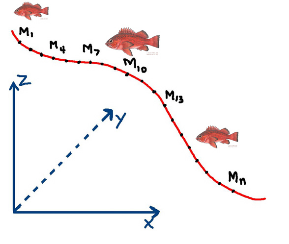
Context of Activities:
Our goal will be to model the transect path of an ROV (remotely-operated vehicle) and
the accompanying video observations that were made. The ROV path and the
observations on that path can be located in the X, Y and Z axes at discrete time
intervals during a dive.
Tutorial Activities
In the instructions below, file names and database objects are in bold;
field names are in italics; menu items are underlined.
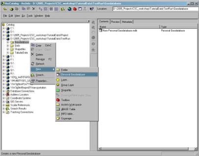
1.0 Building a Personal Geodatabase and Applying the Schema
A. Creating the Geodatabase
- Open ArcCatalog
- Right click the E_Datamodel\Tutorial\Geodatabase folder, highlight
New, then select Personal Geodatabase
- Name it MyArcMarineTut.mdb.
B. Add the Schema Creation Wizard to ArcCatalog
If the Schema Creation Wizard, which looks like this: ,
has already been added, skip to step B.
,
has already been added, skip to step B.
The Schema Creation Wizard is provided in ArcCatalog for loading an existing schema into a blank database. This tool requires an ArcEditor or ArcInfo license to run.
To load it:
- Right click anywhere on the header tool bar and select Customize.
- On the Commands tab, scroll to and select CASE tools, then drag-and-drop the Schema Wizard from the right side (in the Commands window) to anywhere on an existing toolbar.
- Close the Customize window.
What to do if the Schema Wizard does not appear in the tool commands:
- If "Case Tools" does not appear in the list, click "Add from file" and browse to the Bin directory where ArcGIS was installed (usually found in c:\arcgis\arcexe9x\bin).
- Add the Schema.Wiz.dll file.
- If you don't see the SchemaWiz.dll in \arcexe\bin, it may still be there but not
visible. Use Tools/Find File in Windows Explorer to locate the file, and then register the .dll using RegCat.exe, which is also located in \arcexe9x\bin (this too may
also be invisible, follow same steps to locate it). Create a shortcut to the
RegCat.exe on your desktop. Drag the SchemaWiz.dll file onto the RegCat.exe shortcut
and you'll be prompted with a dialog to define where to register the .dll. Select ArcMap, ArcCatalog and ArcTools. Now, when you go to the Categories list you will see
that the Case Tools option is available and the Schema Wizard icon is visible.
C. Applying the Arc Marine Data Model Schema to the Geodatabase
The Schema Creation Wizard will apply existing schemas from two different sources, an XMI file or a repository database. The XMI file is created using a CASE tool (computer aided software engineering) application such as Microsoft Visio 2002. The database repository is a Microsoft Access database containing the desired schema. The Arc Marine Data Model is available in either an XMI or repository; you will be using the XMI format. Note, however, the XMI (XML Metadata Interchange) is a standard that specifies how to store an UML (Universal Markup Language) model in an XML (Extensible Markup Language) file; it is actually an XML file that is loaded.
- In ArcCatalog, with the MyArcMarineTut.mdb geodatabase selected, start the Schema Creation Wizard.
- Read the first info screen then click next.
- Select "Model stored in XMI file"
- Browse to "E_Datamodel\Tutorial\ArcMDM", select ArcGISMarineDataModel.xml then click next
- Select "Use default values" then click next
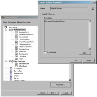
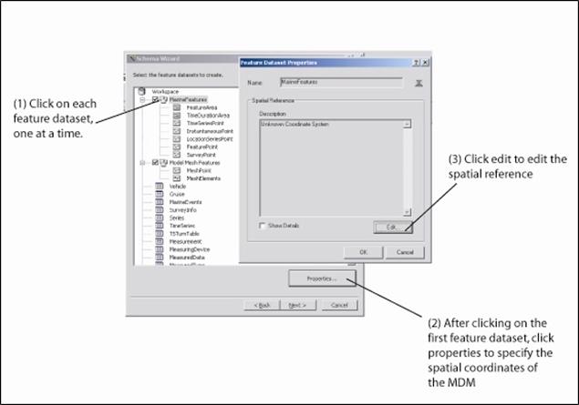
- Review the contents of this schema and their properties. DON'T CLICK "Next" YET!
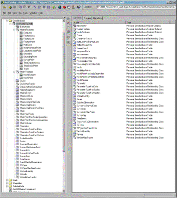
In the hierarchical structure of the geodatabase, you see different objects organized into groups. The objects include:
- The workspace - this is the geodatabase which is a container for geographic data objects
- Tables - called Object classes, store non-spatial objects like equipment specifications or personnel information.
- Feature classes - collections of lines, points, or polygons. Specialized feature classes are used to store annotation, dimension, and route features.
- Feature datasets - container for feature classes (never object classes) that share a common spatial reference.
- Relationship classes - manage thematic relationships between object classes, feature classes, or a combination of the two. They enforce referential integrity between the origin and destination classes.
It is important to have a good understanding of your data structure prior to applying a schema. Because you will be setting parameters that can not be changed later, should you later find that your data does not meet some of the criteria you specified, it will be necessary to rebuild part or the entire schema from the beginning! Feature datasets require that all features within them have the same spatial reference (projection and coordinate system) and are within the bounds of an applied coordinate range (also called domain extent). You will be exploring the specifics of the coordinate range in the next few steps.
- Highlight the MarineFeatures feature dataset
- Click the properties button
Notice that there is no spatial reference
- Click the edit button
The Coordinate system and Domains may be set manually but it is easier to import the spatial reference from an existing layer and modify it to meet your needs. A layer has been provided that is projected to the California Teale Albers projection standard NAD 83. The x/y domain is in the correct range for your data however the m and z domains will need to be modified.
X and Y values are stored for all features. Z and M values are optional values that may be stored with the spatial reference of a feature. Our data contain both Z and M values. The Z and/or M values are stored in the shape field (geometry) of the feature and the option for making a feature "Z" or M aware" can only be set at the time of creation and cannot be changed later. The range of values that can be stored in the X,Y,Z and M reference is set on the Spatial Reference Properties page.
- On the Coordinate Systems tab, Click the Import button
- Browse to E_Datamodel\Tutorial\Shapefiles\Monterey_Study_Area.shp
- On the Z Domain tab, change the Min value to -20000 and Max value to 20000
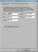
The Z values in your data are stored in meters. Setting this range of values for the Z Domain will allow your data to store the greatest anticipated values (and then some).
Did you notice how the precision changed when you set your range values? Precision is a scale factor that is required to convert storage units to
map units. If you set a precision = 1000 and your data units are meters,
then map units are 1mm or 1/1000 of your data unit. Because the geodatabase
stores coordinates as a positive 4-byte integer, the maximum value is
approximately 2.14 billion map units. The default precision from our imported
spatial reference has a false precision of 100,000 for the M Domain. The
maximum range for storage units that can be stored with this precision is
approximately 21,400 (21,400 * 100,000 = 2.14 billion). Because the M value
units in your data (representing a serial time code) have a range of values
between 0 and 80,000, the default precision will not hold those values, and
thus a precision of 1000 is more appropriate (max value = 2.14 million).
In many cases the default precision is fine; however, this is a case to
demonstrate the importance of knowing your data before proceeding.
- On the M Domain tab, change the value in the precision field to 1000.
- Click OK twice.
- Highlight the feature class named Track and click properties
- On the General tab, click the button next to "Spatial Reference: Custom"
- On the M Domain tab, change the precision to 1000
- Click OK
The default precision propagates to all feature classes within and must be changed independently of the feature dataset.
- On the M/Z tab, confirm that both boxes are checked
- Click OK
- Set the Spatial Reference for the Mesh Features feature dataset to match that of Marine Features
- NOW you can click Next
- Click Finish
- You may review the log file if you wish
2. Loading Data into the Geodatabase
A. Comparing Schemas
Now that the basic schema template has been created, you can compare your data and geodatabase schema for compatibility.
- Open a second instance of ArcCatalog
- Arrange both ArcCatalog windows side by side so that they may both be used.
- In the left ArcCatalog directory, right click E_Datamodel\Tutorial\Shapefiles\TracksMZ.shp
- Select properties
- Select the Fields tab
- In the right ArcCatalog directory, right click E_Datamodel\Tutorial\Geodatabase\MyArcMarineTut.mdb\MarineFeatures\Track
- Select properties
- Select the Fields tab
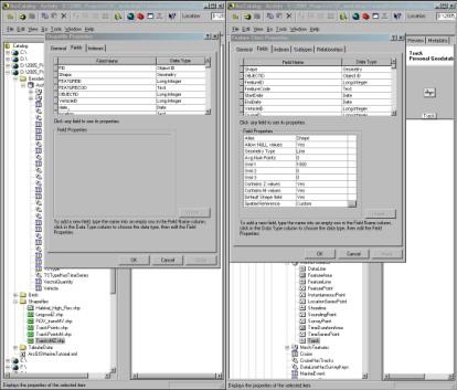
Compare all the fields noting the Data types and Field Properties.
Notice that the geodatabase has an appropriate field to hold all the data
from the TracksMZ shapefile except for the operator field. There are some additional fields in the geodatabase that we will not be using.
Make sure that the database is not being used by any other applications, included the second session of ArcCatalog. You may have to close and reopen ArcCatalog if the database is write protected.
- Scroll down to the bottom of the fields list in the Track feature class
- Click in the first empty row and type Operator
- For data type, select text
- Leave the default values
- Click OK
Compare the schema of
E_Datamodel\Tutorial\TabularData\Monterey2002ROV\Cruise to
E_Datamodel\Tutorial\Geodatabase\MyArcMarineTut.mdb\Cruise
and
E_Datamodel\Tutorial\TabularData\Monterey2002ROV\Vehicle to
E_Datamodel\Tutorial\Geodatabase\MyArcMarineTut.mdb\Vehicle
The schemas match, though not in exactly the same order. When using an existing data model, you will want to collect your data with the model in mind or condition your existing data for the model. A lot of your time will be spent conditioning data.
Close the second instance of ArcCatalog.
B. Loading data
- Right click the Track feature class
- Highlight Load then select Load data
- Browse to E_Datamodel\Tutorial\Shapefiles\TracksMZ.shp
- Click Add, then Next (to skip the subtype loading)
- Click Next
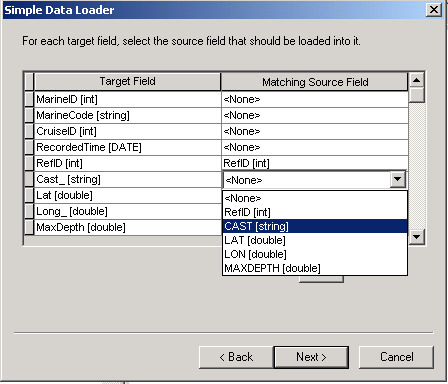
In this window you will be matching the fields from your source data to the fields in your database.
Match the following fields:
| FeatureCode [string] | | FeatureCod [string] |
| StartDate [DATE] | | date_[DATE] |
| EndDate [DATE] | | date_[DATE] |
| TrackID [int] | | FeatureID [int] |
| Name [string] | | None |
| Method [string] | | None |
| Description [string] | | None |
| LocalDesc [string] | | Location [string] |
Example from another application:
- Click Next
- Confirm that "Load all of the source data" is selected, click next
- Click Finish
- Preview the Track feature class geography and table in ArcCatalog
Notice the shape records indicate Polyline ZM, showing that this layer is both Z and M aware.
- Load both the Cruise and Vehicle tables from E_Datamodel\Tutorial\TabularData\Monterey2002ROV.mdb
- Load E_Datamodel\Tutorial\Shapefiles\Coastline_mb.shp into the Shoreline feature class. Do not match any fields.
C. Importing Objects
Classes (object or feature) may be imported directly into the geodatabase. This is a very easy way to modify schema.
- Right click MyArcMarineTut.mdb, highlight Import, then select Table (Multiple)
- NOTE: This function may NOT
work properly in v. 9.2 or v. 9.3! A work-around is to use the Import Table (Single)
function instead.
- For the Input table, browse to E_Datamodel\Tutorial\TabularData\
Monterey2002ROV.mdb and select both the SpeciesObservation and
HabitatSegments tables
- Click Add, then OK
- Verify that the tables are now in your database.
- Right click the MarineFeatures feature dataset, highlight Import, then select Feature Class (single)
- For "Input Feature", browse to E_Datamodel\Tutorial\Shapefiles\
Habitat_High_Res.shp. For "Output Feature Class Name," type HabClass
- Click OK.
- Verify that HabClass is now a feature class in MarineFeatures
D. Creating a Raster Catalog
Raster data may also be loaded into your geodatabase as a raster object or contained in a Raster Catalog. A raster catalog allows you to manage multiple rasters as if they were tiled together (mosaic). With personal geodatabases the raster is not actually stored within the .mdb file. (This is good because the .mdb is limited to 2GB!). Instead the files are converted to IMG format and stored in a directory that rides along with the geodatabase. If the rasters are "managed" then this directory will be moved anywhere the geodatabase is moved when using ArcCatalog. For this reason, it is important to never move personal geodatabases containing raster data using Windows Explorer.
- Right click MyArcMarineTut.mdb, highlight "new", then select "Raster Catalog"
- For "Input Raster Catalog Name" type Bathymetry
- To set the "Coordinate system" for the raster", click the button
- Import the coordinate system from the Monterey_Study_Area.shp using the same method as for the feature datasets
- Set the "Coordinate system for the geometry column" field using the same
- Click OK
E. Loading Rasters into a Raster Catalog
- Preview the defined projection for E_Datamodel\Tutorial\Grids\c_p2mhill
and E_Datamodel\Tutorial\Grids\m_c2mhill
- Right click the new Bathymetry Raster Catalog, highlight load,
then select Load Data
- For "Input Rasters" browse to E_Datamodel\Tutorial\Grids and select
c_p2mhill and m_c2mhill
- Click Add then OK... this will take a couple minutes... shouldn't be more than a couple.
- NOTE: These steps may NOT
work properly in 9.2 or 9.3! A work-around is to try loading m_c2mhill and m_c2mhill into ArcMap in Step 4A below as needed.
- Preview the Bathymetry Raster Catalog - both rasters are shown as a mosaic
- Select the Contents tab
- Click on the handle to the far right (it has two black triangle on it)
- Next, click on the handle at the bottom left
- In the query type [OBJECTID] = 1 (you should see the c_p2mhill grid appear)
- Click Selection
- Click Subset... compare Selection and Subset options.
- In the query type [OBJECTID] = 1 or 2
- Click Selection
- In the window in the very lower right of ArcCatalog, change the selection
from "Geography" to "Properties"
- In the Contents window, scroll down to "Spatial Reference"
Notice that the spatial reference of the raster has changed. The geodatabase will reproject data to match the raster catalog.
3. Creating Relationships in the Geodatabase
A. Creating Relationship Classes
Now that all of our data are in the geodatabase we can create relationship classes that link our data together.
- Right click the Track feature class, select Properties
- On the Relationships tab, Highlight the relationship CruiseHasTracks, then click Properties
Notice this relationship links Cruise and Track with a one-to-many (1-M) relationship. The tables are linked through the key fields CruiseID.
Click cancel twice
Right click MyArcMarineTut.mdb, highlight New, then
select Relationship class.
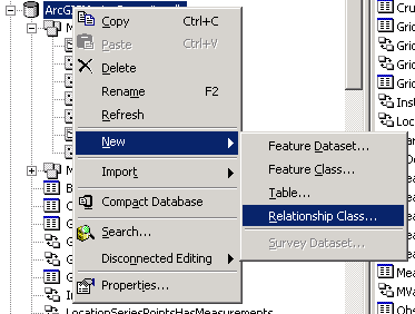
Another example:
- In the "Name of the relationship class" field type VehicleHasTracks
- Select Vehicle for the origin table and Track for the
destination table
- Click Next
- Select "Simple (peer to peer) relationship" then click Next
- Accept the default labels, click Next
- Select 1 - M (one to many) then click Next
- Verify "No" is selected and click Next
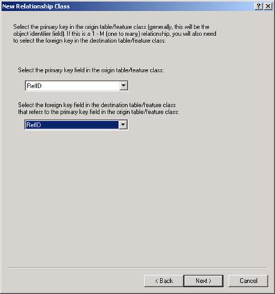
- Select VehicleID for both the primary and foreign keys then click Next
- Click Finish
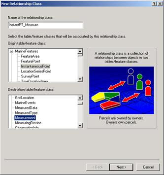
- Create a new Relationship Class and call it TrackHasObservations, using Track and SpeciesObservations as your origin and destination tables.
- Continue with the same parameters as above except the primary key is
FeatureID and the foreign key is SegmentID.... Pay close attention
to the order of cardinality (which is the one and which is the many?)
Your geodatabase is done! We will now explore the data and how they relate. Part of your exploration will cover a brief overview of dynamic segmentation. Dynamic Segmentation will link the habitat and species observations to their proper geography using the M values stored in the Track geometry.
4. Adding Geodatabase Features to your ArcMap Project
A. Adding and exploring the data
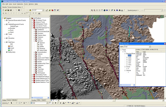
- Open ArcMap, and add the following data from MyArcMarineTut.mdb: Track, Shoreline, HabClass, Bathymetry, HabitatSegments, and SpeciesObservation
- Notice that HabitatSegments and SpeciesObservations are stored in object classes (no geometry).
- Spruce up the display of HabClass by right clicking on the layer and choosing Properties and within Layer Properties: Display (set transparency to 50 or 60%); in Symbology (show Categories in Unique Values, Value Field of "IND", Add Values of "hard", "mixed", "soft", giving them nice colors)
- Save your ArcMap document to E_Datamodel\Tutorial\MyGDB_Tutorial.mxd
In ArcCatalog:
And your ArcMap session should look something like this: (although this screen shot also shows the dynamic segmentation referencing that you will do in the next steps)
In order to spatially display the HabitatSegments and SpeciesObservations data, you will reference the data using dynamic segmentation. Dynamic segmentation is the process of transforming linearly referenced data (called events) stored in a table into a feature that can be displayed on a map. The habitat and fish observations contain an integer ID that is the serial time code for when the observation took place on the ROV transect. The M (measure) value that is stored in the spatial reference of the Track feature is the serial time code.
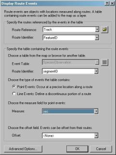
In ArcMap you can "Display Route Events" to view these data spatially.
- In the Table of Contents, right click HabitatSegment then select Display Route
Events
- For Route Reference select Track
- For 1st Route Identifier field, select FeatureID
- For 2nd Route Identifier field (under "Specify the talbe containing the route events), select SegID
- Change the type of events to "Line Events"
- In the From-Measure field select BTCsec
- In the To-Measure field select ETCsec
- Click OK
- As you did above for HabClass, change the symbology of the HabitatSegments Events layer to show the unique values of the Habitat Type field
- Right click SpeciesObservation and display the route events...
SegmentID is the table Route identifier; the events are point; set the
measure field to sec
- You may select and create a layer for a specific species if you wish (the attribute is "COMNAME")
B. Propagating relationships
- Turn off any Species layers
- Zoom into the map until you can see individual tracklines from the Track
layer
- Click the main Selection menu and set the selectable layers to Track
- Using the Selection tool, select a trackline of interest
- Right click the Track layer and open the attribute table
- Click the Selected button at the bottom of the table
- Click the Options button, highlight Related Table then
select TrackHasSpObservation: SpeciesObservation
- Rearrange the windows so that you can see the attributes of
SpeciesObservation as well
- Click the Selected button at the bottom of the table
Notice that the SegmentIDs of the selected records in the SpeciesObservation table
match the FeatureIDs of the selected records in the Track table. The record selection
has been propagated through the relationship classes in the geodatabase.
For the trackline of interest that YOU chose, use the other related tables to answer:
- On which cruise did this track take place?
- What vehicle made this track?
5. Exploring the Z-Value - Optional
If you're interested in displaying the z-value geometry for the tracklines
and observations, open the E_Datamodel\Tutorial\Tutorial3D.sxd file.
Because ArcScene doesn't support dynamic segmentation, shapefiles have been
exported from the geodatabase for you to show observational features.


